Tutorial: Plot RADAR data using GrADS

GrADS is great for plotting model data, but did you know that you can plot RADAR and satellite data as well?  This tutorial is very similar to the plotting satellite tutorial, and will take you through the steps of making plots with archived RADAR data from the National Climatic Data Center (NCDC).

For this tutorial, it is recommended that you use the script color.gs and cbar.gs.  Alternatively to color.gs you could use the script colorset.gs to approximate the NWS RADAR color scale.

Using GrADS to plot radar data is not much different than using GrADS to plot model data, and is essentially compromised of three main steps.

1. Get RADAR data
2. Save data into a netcdf file
3. Plot the data using Grads

Step 1: Get the Data.

You can download archived RADAR data from the NCDC at this website.
Accessing the data is very simple, and only requires you to pick a RADAR site and time.  Enter your e-mail address into the box provided and a data request number will be sent to you shortly after.

You can additionally download data in real time via FTP from this website.  I have had success using a batch version of NOAA's weather and climate tool kit data exporter.  More information on this can be found here.

However assuming that you are downloading archived RADAR data, you can simply use the online version of the weather and climate toolkit here.  Once you have this program open on your computer, it is time to move on to step 2.

Step 2: Convert the Data to Netcdf Format.

Once you have both the toolkit and the data request number, you can now access the data.  Accessing the data is simple, all you have to do is choose the "load data" option to bring up the "data selector" window.  Once this window is open, choose the tab NCDC HAS Order and enter your confirmation number into the space provided.

NCDC Weather and Climate Toolkit

Once you have your list of files, choose the "export" option.  This will bring you to another list of options to go through.  Choose "gridded netcdf" as your file type, after that the options are pretty much up to you.  I generally just click through keeping the default options.

Once the program is finished processing the data, you will see a file in your folder that looks something like this:KVWX_NCR_20100510_162700.nc.  Basically, the name is made up of the RADAR call sign, the variable, the date and the time.  This file is a self describing netcdf file, and can be read into GrADS.  Which brings us to the final step.


Step 3: Plot the data in GrADS

First open your file using the 'sdfopen' command.  Once the file is open, you can follow the commands listed below to approximate the standard RADAR color scheme used in operation by NOAA using color.gs.

     'set gxout grfill'
     'set mpdset hires'
     'color 5 75 5 -kind dodgerblue->blue->lime->green->darkgreen->yellow->goldenrod->orange->firebrick->red->darkred->fuchsia->indigo
     'd cref'
     'cbar'

...or alternatively, using colorset.gs:

      'set gxout grfill'
      'set mpdset hires'     'colorset Rad1'
     'd cref'
     'cbar'

Another option for a RADAR color scheme that approximates the standard NWS scheme (available from COLA. Full example here) is listed below as a function.  It is called as such:

     getcols()
     'set ccols 20 21 22 23 24 25 26 27 28 29 30 31 32 33' 
     'set clevs 5 10 15 20 25 30 35 40 45 50 55 60 65 '

    function getcols()
    'set rgb 99 140 140 116'
    'set rgb 20 180 200 255'
    'set rgb 21 95 135 255' 
    'set rgb 22 20 70 230' 
    'set rgb 23 110 245 75' 
    'set rgb 24 0 195 0' 
    'set rgb 25 0 115 0' 
    'set rgb 26 255 255 0' 
    'set rgb 27 255 180 48' 
    'set rgb 28 250 125 0'
    'set rgb 29 230 45 0'
    'set rgb 30 175 0 0'
    'set rgb 31 105 0 0'
    'set rgb 32 250 0 200' 
    'set rgb 33 155 0 250'

No matter which color scale you use, your resultant image should look similar to the one below.

Example of RADAR data from GrADS

Download this script

Read More

Tutorial: Draw Sea Level Pressure map with labeled Hi/Lo pressure centers using GrADS

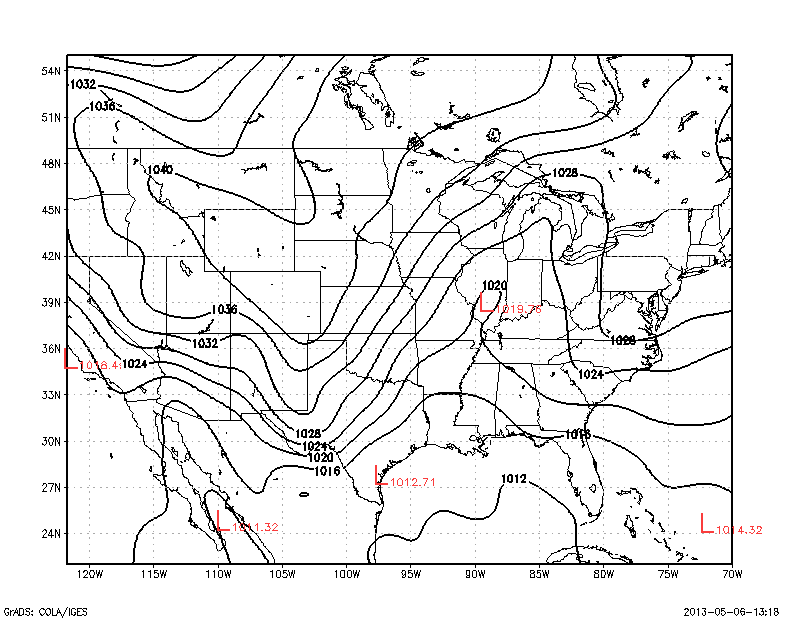
Maps of sea-level pressure just don't seem complete without little red "L's" and blue "H's" marking the pressure centers.  However, marking these locations in GrADS can be quite burdensome.  This tutorial will teach you how to use the mfhilo function from the library of functions from Mike Fiorino made available in the newer versions of GrADS (v1.1 and newer) to plot H's and L's on a SLP map.

Before

After

Plotting a map of sea-level pressure is easy, and follows the basic commands.  For the image above, we will set the appropriate domain and use a polar-stereographic map projection.  The following commands set up the domain, open the data file and plot the sea-level pressure.

     'sdfopen http://nomads.ncep.noaa.gov:9090/dods/gfs_hd/gfs_hd20130502/gfs_hd_12z'

     'set display color white'
     'clear'
     'set map 1'
     'set mpdset hires'
     'set mproj nps'
     'set lat 20 55'
     'set lon -140 -60'

These commands by themselves will give you the "Before" image.  Now the tricky part, using the mfhilo function, and grabbing the pressure centers.

the mfhilo function is another one of those functions that works with arguments.  A full list and description of the different options can be found here.  For the example here, I will use the contour level method to find maxima/minima in the sea-level pressure field.  Basically, this method uses looks for minima/maxima that cross certain thresholds and are certain distances apart from other minima/maxima.  You can tweak the threshold values as desired to get the right number of marks on your plot.  Through trial and error I have found that a Radius of ~1000 and a contour interval of ~300 works fairly well with SLP maps.  So the command to find low pressure centers is:

     'mfhilo prmslmsl/100 CL l 1000, 300'
     say result

The preceding commands will output this to the screen:

    mfhilo CL method N: 4  maxmin: -1   radinf:  1000.0 [nm]   cintinf:   300.0  lat
    c:  37.50 lonc: -100.00
    L    21.97  -90.35  M:    1009.81  D:  1829.44
    L    24.88 -109.54  M:    1011.32  D:  1056.93
    L    21.26  -70.10  M:     1013.5  D:  597.76
    L    39.05  -89.04  M:    1019.76  D:  524.40

Now we have salient information about four low pressure centers: Lat, Lon, and Value.  So, now getting this data printed to the screen is only a matter parsing this information.  The first thing we will do is save this information into a new variable.

   Low_info=result

Now, we have the information saved, we need to run through each minima.  We can do this through a conditional loop, checking to make sure that the first word of the each line is an L.  Then simply count through each line until this condition is not met.  So our code to draw L's all over the map looks like this:

     i=2         ;*Since the data starts on the 2nd line
     while(subwrd(minmax,1) = 'L') 
       min_lat = subwrd(minmax, 2)
       min_lon = subwrd(minmax, 3)
       min_val = subwrd(minmax, 5)

      'q w2xy 'min_lon' 'min_lat  ;*converts lat/lon to page coordinates
      x_min = subwrd(result,3)   ;*finds page coordinates for x
      y_min = subwrd(result,6)   ;*finds page coordinates for y


        'set strsiz .28'
        'set string 2 c 9'
        'draw string 'x_min' 'y_min' L'
       
        'set strsiz 0.1'
        'set string 2 bl 2'
        'draw string 'x_min+0.1' 'y_min-0.15' 'min_val

      i=i+1
      minmax = sublin(Low_info,i)
endwhile

However, this is not good enough.  I tweaked some of the domain settings to show why this is an issue, but often times, these maxima/minima will occur near the edge of the plot, and the L's and H's can get drawn overlapping the map border, which is just messy looking.  An example is shown below.

Example showing data plotted off of the map.

To get around this, you must input an "invisible" boundary that keeps the script from plotting L's too close to the edges.  There is more than one way to do this, the way that I do it is by replacing the block of code that draws the L's with this:
 
     'q gxinfo'
     xline=sublin(result,3)
     yline=sublin(result,4)
     xs=subwrd(xline,4)' 'subwrd(xline,6)  ;*Gets x boundaries
     ys=subwrd(yline,4)' 'subwrd(yline,6)  ;*Gets y boundaries
   
*    Conditional Statement requiring the L's be some distance away from the plot boundaries.

      if(y_min > subwrd(ys,1)+0.1 & y_min < subwrd(ys,2)-0.1 & x_min > subwrd(xs,1)+0.1 & x_min < subwrd(xs,2)-0.5)
        'set strsiz .28'
        'set string 2 c 9'
        'draw string 'x_min' 'y_min' L'
       
        'set strsiz 0.1'
        'set string 2 bl 2'
        'draw string 'x_min+0.1' 'y_min-0.15' 'min_val
      endif
 
By doing this, you prevent messy plots with L's and H's plotted outside of the page area.  With this correction, the previous plot now looks like this.

Corrected, with invisible boundaries

Once you have plotted the L's you need to plot the H's.  This requires essentially the exact same block of code, only now the mfhilo function looks for maxima instead of minima, and you change the color of your plotted letter.  When it put it all together, you get this long chunk of code here:

*   ******************************DRAW L's******************************

  'mfhilo prmslmsl/100 CL l 1000, 300'
  Low_info=result
  i=2         ;*Since the data starts on the 2nd line
  minmax=sublin(Low_info,i)

  while(subwrd(minmax,1) = 'L')

    min_lat = subwrd(minmax, 2)
    min_lon = subwrd(minmax, 3)
    min_val = subwrd(minmax, 5)

    'q w2xy 'min_lon' 'min_lat      ;*Translate lat/lon to page coordinates
     x_min = subwrd(result,3)
     y_min = subwrd(result,6)

    'q gxinfo'                      ;*Get area boundaries
    xline=sublin(result,3)
    yline=sublin(result,4)
    xs=subwrd(xline,4)' 'subwrd(xline,6)
    ys=subwrd(yline,4)' 'subwrd(yline,6)

    if(y_min > subwrd(ys,1)+0.1 & y_min < subwrd(ys,2)-0.1 & x_min > subwrd(xs,1)+0.1 & x_min < subwrd(xs,2)-0.5)
      'set strsiz .28'
      'set string 2 c 9'
      'draw string 'x_min' 'y_min' L'
       
      'set strsiz 0.1'
      'set string 2 bl 2'
      'draw string 'x_min+0.1' 'y_min-0.15' 'min_val  ;*Plots value to the lower right of the L
     endif

    i=i+1
    minmax = sublin(Low_info,i)
    endwhile

*   ******************************DRAW H's******************************

   'mfhilo prmslmsl/100 CL h 1000, 300'
    High_info=result
    i=2         ;*Since the data starts on the 2nd line
    minmax=sublin(High_info,i)

    while(subwrd(minmax,1) = 'H')

       min_lat = subwrd(minmax, 2)
       min_lon = subwrd(minmax, 3)
       min_val = subwrd(minmax, 5)

       'q w2xy 'min_lon' 'min_lat      ;*Translate lat/lon to page coordinates
       x_min = subwrd(result,3)
       y_min = subwrd(result,6)

       'q gxinfo'                      ;*Get area boundaries
       xline=sublin(result,3)
       yline=sublin(result,4)
       xs=subwrd(xline,4)' 'subwrd(xline,6)
       ys=subwrd(yline,4)' 'subwrd(yline,6)

       if(y_min > subwrd(ys,1)+0.1 & y_min < subwrd(ys,2)-0.1 & x_min > subwrd(xs,1)+0.1 & x_min < subwrd(xs,2)-0.5)
         'set strsiz .28'
         'set string 4 c 9'
         'draw string 'x_min' 'y_min' H'
       
         'set strsiz 0.1'
         'set string 4 bl 2'
         'draw string 'x_min+0.1' 'y_min-0.15' 'min_val  ;*Plots value to the lower right of the H
       endif

       i=i+1
       minmax = sublin(High_info,i)
     endwhile

So the code for this is kind of long, but most of it is translating lat/lon to page coordinates so that you can draw your L's and H's in the right place, and so that you don't plot them too close to the edges of your plot.  But now you are all set to make sea-level pressure maps with L's and H's'  Like I said, a radius of 1000 and a contour interval of 300 usually is a good balance between too many and too few marks, it's best for you to experiment with it until you come to a few settings you are comfortable with, so in the downloadable script, I set these two variables at the top so you can change them around easily.

Download this script






   

Read More

Tutorial: How to save data into a .txt ascii file using GrADS; Example: Gridded Temperature Data

Note: This tutorial has been updated in October 2019 to reflect the fact that the GDS has been discontinued.  The general principles of this tutorial have not changed, but now you need to download a small data file to your local computer to follow the tutorial.
Since GrADS cannot easily perform high level data analysis techniques, (barring a few complicated workarounds) it is useful to save data so it can be used with more advanced software.  While it is often logical to skip GrADS altogether, it can occasionally be easier to use GrADS as an intermediary step since it's a very intuitive scripting language for gridded datasets.

This tutorial will teach you how to save data using GrADS using the "write" function by guiding you through an example that will save latitude/longitude and monthly average surface temperature data from NCEP reanalysis into a .txt file.

Okay, so as always we will need to start by opening at data file.  For this tutorial, I am using the monthly mean 2 meter air-temperature reanalysis product.  To follow this tutorial, you will need to download the "air.mon.mean.nc" file from the ESRL PSD NCEP 1 Reanalysis website.  Once you download the file, and save it to your data directory, open the file in GrADS using "sdfopen"

  'sdfopen /home/your_datapath/air.mon.mean.nc'

Again, you are welcome to query the file to look at some of the metadata, but it's not required that you do so.  It is however good practice to plot the data and make sure it looks resonable before proceeding.  This dataset spans a long range of time, and for this tutorial, I am going to randomly choose February 2000 as the time value.  To specify the date instead of the timestep when picking a time, use the 'set time' (as opposed to 'set t') command.  Note that the time format must be %hhZ%dd%MMM%yyyy as in the example  below.

     'set time 00Z01FEB2000'
     'set gxout shaded'
     'd air'

Mean 2m air temperature from Feb 2000

Now that we have an idea what the data looks like on a map, we can move on to saving it into a .txt file.  Saving data from GrADS into an outside file is actually pretty straightforward.  The hard part is figuring out how to organize each piece of data exactly how you want it.

The first thing to do is to determine what data we would like to save, and how to organize it.  I find it a good practice to include the x/y grid indices when saving data into a text file.  So, the final text output will have five data columns, the x/y grid point indicies, the lat/lon value at each grid point, and the actual temperature data.  It's also good practice to include a header line at the top of the text file to specific which column is which.  So, the first step is to open the file and write header.  This is done by using the "write" function in GrADS.

     write('NCEP.txt', 'X    Y    LON    LAT    TEMP')

Once this command is executed in GrADS the file NCEP.txt will be created in your folder with the text "X    Y    LON    LAT    TEMP" on top.

Now that the data file has be started, it's time to start filling it up with data.  To do this, you need to set the GrADS  output to write our data out to the screen instead of plot it on a map.  This is done by setting 'gxout' to print.  In addition to that, you need to specify how GrADS should format our printed data.  This is done with the 'prnopts' command using C formating syntax.

     'set gxout print'
     'set prnopts %6.2f 1 1'    ;*%6.2f: c format, 1: values to plot on each line, ;space between values

Now that GrADS is set to print to the screen, and the print formatting is set, you are now ready to save the data.  The way to do this is to loop through all the grid-points and save the data to the file one grid-point at a time.  In this example, the nested loop to do this will first run across the x (longitude) direction, then through y (latitude), saving the information into rows as we go.  To begin, we will first need to set limits on our domain so that the loops know when to stop.  Do this by the use of the 'query' function

     'q dims'
     xline=sublin(result,2)    ;* 2nd line
     yline=sublin(result,3)    ;* 3rd line

     xmax=subwrd(xline,13)    ;*13th word on xline
     ymax=subwrd(yline,13)    ;*13th word on yline

     say 'X grid-points: 'xmax
     say 'Y grid-points: 'ymax
   
This code will print out the following to the screen:

   X grid-points: 193
   Y grid-points: 94

Now that domain dimensions are known, you can initialize the loops.  There is very little code within the nested loop.  First the 'display' command (which because of the 'gxout' and 'prnopts' configuration described above) is used to print out the temperature data at each grid-point to the "result" variable.  To save the data to the file, the only thingsleft to do are a) pull the temperature from the results data, b) pull the lat/lon values using the 'q dims' command, and c) write the data to a new row in the NCEP.txt file.  The code is as follows:

     y=1
     while(y<=ymax)
        x=1
        while(x<=xmax)
           'set x 'x
           'set y 'y
           'd air'

     * NOTE: It may be useful to test this to find out where the data is contained with in the result
     * It just so happens that in this case, the data is the 1st word of the 2nd line, this is not always true

           tmp=sublin(result,2)
           tmp=subwrd(tmp,1)

    *Get Lat/Lon Data
           'q dims'
           lons=sublin(result,2)
           lats=sublin(result,3)
           lon=subwrd(lons,6)
           lat=subwrd(lats,6)

    *Save data to file
    *Note the "append", so to add to the file instead of overwriting it
           write('NCEP.txt', x'    'y'    'lon'    'lat'    'tmp, append)
           x=x+1
      endwhile
      y=y+1
   endwhile

That's actually all there is to it.  This script will take a few moments to loop through all of the grid-points, and as it does so you will likely see the words "unknown command 0" printed a bunch of times on your screen.  I have often found it helpful to include a "say" command inside the loop, so to know where I am in the saving process.  When this script finishes you will have a lot of data saved into a .txt file that can be read into any plotting or statistical program.  For example, to confirm GrADS saved the data correctly to text, I created the image below by loading NCEP.txt into a Python array and plotted it on a map using Matplotlib and Cartopy.

NCEP.txt data plotted using Cartopy

As always, I included a downloadable script for this tutorial: Download this script

Note: The downloadable script has not been updated since it was originally created, and will therefore not work when trying to access the GDS.

Read More

Tutorial: How to make a basemap using GrADS

Note: This tutorial was updated October 2019 to reflect the fact that the Grads Data Server has been discontinued, so the online access of the terrain data through monsoondata.org is no longer available.

This tutorial was first published in 2013, with a tutorial on how to create a basemap of the United States.  In updating the tutorial for 2019, I have decided to alter the tutorial to focus on a different region of the globe, Europe to be specific.  Functionally, the concepts are the same (see images below).

Introduction:
Basemaps are a great way to add some color and vibrance to your weather maps.  GrADS allows you to output data onto a pre-generated .png image (i.e., a basemap) instead of redrawing the map everytime you want to make a figure.  This can be a big time saver if you're making several images in sequence.  This tutorial will show you how to make a basemap in GrADS using the 'basemap.gs' script and accompanying polygon files to mask the ocean..  You will learn how to:

1. Download and open netCDF topography data from NOAA 
2. Use the and the "basemap" script from the GMU GrADS Script Library to mask out oceans. 

It is recommend that you check out the basemap overlay tutorial if you are unfamiliar with GrADS basemaps.

Finished Basemap: 2013 Tutorial

Finished Basemap: 2019 Tutorial

So, for this tutorial you must download the following files from the GMU GrADS Script Library.

• basemap.gs
• lpoly_lowres.asc
• opoly_lowres.asc
• lpoly_mres.asc
• opoly_mres.asc
• lpoly_hires.asc
• opoly_hires.asc

In addition to these scripts, it is recommended that you have the color.gs and/or the colormaps script your personal script folder so you can use the same color settings as this tutorial.

Where to get the data:
While the GDS has been discontinued, you can still access high resolution (1min) topography datasets in netCDF format from NOAA.  Simply access this link and download either the full ETOPO1 (netcdf) file, or use the NCEI "Grid Extract Tool" to subset the data to a geographic region of your choice.  If you're using the Grid Extract Tool it will look similar to the screen shot below.

Screen shot of grid extract tool.

Once you have the netCDF (etopo1.nc) file locally, move it to your own data folder: (e.g., home/grads_data/terrain/).

How to make the basemap:
Basemaps are fairly easy to make, and can essentially be boiled down to three simple steps.

1. Load the topography data and set a domain.
2. Define a topography color scale (this is why we need color.gs)
3. Fill in the water areas using the ".asc" files

Step 1: Load the topography data and set a domain:

This is probably the most important step in making a basemap.  In order to use the basemap later for your weather maps, you must know a) The lat/lon boundaries, b) the size of the image in pixels, and c) the GrADS page area of the map (set using the 'parea' command).  I strongly recommend that you write down your lat/lon boundaries, your page area coordinates,and your x and y pixel size for saving the image so that you know how to match data on top of the map.

    'set display color white'
    'set mpdset hires'
    'clear'
    path = 'home/grads_data/terrain/' ; *or whatever your path to the etopo1.nc file is.
    'sdfopen 'path'etopo1.nc'

You can run a "qfile" on the data to look at the metadata if you would like, but it's not necessary for this tutorial.

Now to set the actual domain.  So, to make the image above, we will set the domain for the United States.  We will do this using the 'set lat' and 'set lon' commands.

  'set lat 30 60'
  'set lon -16 35'
At this point, we have our file open and our domain set.  So the last thing we need to do before moving on to step 2, is define our page area.  Remember this is important, so you know how to scale your weather maps in GrADS to fit on this image.  We do this using the 'set parea' command.  For the above image, the page area is set by:

   'set parea 0.5 10.0 0.5 7.5'

Now that we have our area, we can move on to step two.

Step 2: Define a Topography Color Scale

This is very easy with the color.gs script, all you need to do is pick out a range of colors.  For the old US map, we used the color.gs script to make a color scale that transitioned from light green to brown, that fit the range of topography in the US (0 to ~4000 meters).

    int=(4100-200)/50       ;*int sets the interval used for topography, this scale sets 50 intervals.
    'color 200 4100 'int' -kind lightgreen->tan->brown'

For the 2019 update, I chose to use the colormaps script to define the "terrain2" color scale as follows:

  'colormaps_v2 -map terrain2 -levels 0 3500 100'

Choosing a color scale is entirely, up to you, but the above options look nice to me.  Once the color scale is set, simply display the variable.


Now, our basemap is starting to take shape and we are set to move on to the final step.

Step 3: Fill in Water areas
This is the last step, and the only step that involves the use of basemap.gs.

To fill in the water areas, you will need to run the basemap.gs script as such:

    'basemap O 11 1 M'

In this command, the O stands for Ocean, so the script will fill in bodies of water.  The two numbers correspond to the fill and outline colors respectively.  11 for medium blue and 1 for black.  Lastly, the M stands for medium resolution, so this will use the file opoly_mres.asc to fill in the ocean.  The reason to use mres instead of hires, is because the hires oceans only cover the oceans around North America, so since this tutorial looks over at Europe, you need to use mres.

Now, that you have a nice looking basemap, all thats left is to save the image using the 'printim' command.  Be sure to specify the image dimensions, so that you can match them later when you save GrADS output over your basemap.

    'printim img_name.png x800 y600 png'

And that's it, that's all there is to it! You now have a nice, elegant basemap to serve as a background for your GrADS output.  To learn more how to output GrADS data onto your basemap, check out this tutorial.

Note: This example script is for the 2013 tutorial with the broken GDS link.

Download Example script

Read More

Tutorial: Overlay image on basemap image using GrADS

This tutorial teaches you how to save GrADS output onto an already existing image, a basemap.  This allows you to bring more color and vibrance to your weather map by adding, for example, topographic maps underneath of your weather data.  The use of basemaps can transform the image on the left to the image on the right.

Before Basemap

After Basemap

Before we get started with the tutorial, it is recommended that you learn how to make your own basemaps (see tutorial on making basemaps here).  However, if you want to skip learning how to make basemaps for now, I will provide the basemap needed for this tutorial.  The basemap provided will be the same basemap used in the above example.  To download this basemap to your computer, simply right click on the image below and choose "Save Image As..." and save it to your GrADS folder.

Save this image, as your basemap for this tutorial

So, now that you have your basemap, lets get started.  Plotting data onto a basemap is very simple, and requires very little extra code.  All you need to do is add a few extra options onto the 'printim' command, when you are outputting your data to an image.

• Normal: 'printim img.png png x800 y600'
• Basemap: 'printim img.png png x800 y600 -b basemap.png -t 0'

The options -b and -t, respectively, stand for 'basemap' and 'transparency'.  After the -b you must indicate the path to the basemap image, and after the -t you must specify which color to make transparent.  You can find out this number by querying the shading information through the 'q shades' command, or simply specifying this number through the 'set ccols' and 'set clevs' command.

And that's pretty much all there is to overlaying your data onto a basemap.

There are however a few things to watch out for.  Since all you are essentially doing when you include the -b option, is printing your GrADS plot onto a preexisting image, you need to make sure all the image dimensions match.  To do this there are really only three things that you need to remember:

1. Your GrADS page area (parea) matches the page area on your basemap
2. Your image dimensions are equal (you can get your image dimensions by right clicking your image and looking at 'properties')
3. Your lat/lon boundaries must be the same between the basemap domain and the GrADS domain

If these three conditions are not satisfied, you will end up with an overlay that does not coincide with your basemap (see below image for an example of what this looks like)

Incorrect!

Now, that you have an idea on how to do it, here are the correct dimensions for the basemap provided here.

Image Dimensions: x=800px, y=600px
Parea: '0.5 10.0 0.5 7.5'
latitude: 22, 51
longitude: -128, -65

So if you were to use these dimensions in a script to plot radar, your code might look like:

     'set mpdset hires'
     'set lat 22 51'
     'set lon -128 -65'                                                        ;*Depending on the dataset, you may need to add 360 to this
     'set display color white'
     'clear'

     'set parea 0.5 10.0 0.5 7.5'                                                  ;*Note the page area is equal to the basemap
     'set gxout shaded'
     'set ccols 0 14 4 11 5 13 19 7 12 8 2 6'                                ;*Note that the 0 is the specified transparent color
     'set clevs  5 10 15 20 25 30 35 40 45 50 55 60 65'
     'd radar'
     'printim img.png png -b basemap.png -t 0 x800 y600'       ;*x800, y800 correspond to the image dimensions


That about does it for this tutorial, you should now be able to overlay images onto preexisting basemaps.  And just for fun, and so you know, your background image does not necessarily have to be a map.

I hope you enjoyed, and found this tutorial useful!

 Download example script

Read More

Tutorial: Basics of Scripting

This tutorial is short and focuses on the very basics of GrADS scripting.  It is the goal of this tutorial to provide a little background on scripting and to help the budding GrADS user avoid various (and frustrating) syntax pitfalls often encountered while scripting with GrADS.

Why Script?  Easy; because it's annoying to keep typing the same commands over and over in the console. Scripting allows you to place all of your commands in one file, and then execute a number of GrADS commands in sequence with a single command.  Additionally, scripting allows you to further extend the capability of the GrADS software; for example you can use tools such as mathematical functions, conditional statements and loops within a script, whereas you cannot use these tools using the command line.  There are however a few important syntax issues that differ when using scripting vs. using the command console.

How to start a new GrADS script:  It is straightforward to start a new GrADS script.  All you need to do is open up a text file and start adding various GrADS commands to it, in the order that you wish to execute the commands.  When you want to run the script, simply save it with the suffix ".gs", If you are using Windows, be sure to change the "save as" option from ".txt" to "all files", and use the ".gs" suffix.  To run the script in GrADS, open GrADS, and type in the name of the script (be sure to include the path if it is in a different directory than the one you are running GrADS out of).

Scripting Basics: How to avoid syntax errors when writing your GrADS Script:  The following list is designed to help you learn some of the basic syntax involved in using GrADS commands within a script.  Because scripting allows you to use functions, and variables that fall outside of the basic GrADS command structure, you must be able to distinguish GrADS commands within your script.  Below is a list of several syntax quirks and methods used in the GrADS scripting format.

• GrADS commands must be inside single quotes (')
• Variables must be outside of the single quotes
• NO indentations are allowed, avoid the TAB button keep at all costs
• Lines can be commented out using the astrix  (*)
• Note: When commenting the * must be on the farthest left column of your text

• Semi-colons (;) can be used in place of a new line
• The results of queries are put into the default variable 'result'
• Concatenating (adding) strings is easy, just type them in sequence
• e.g., str1='Hello' and str2='World': str1' 'str2 outputs as 'Hello World'

• Mathematical operations involving control file variables occur inside single quotes (')
• For example, converting Temperature in C to F would look like 'temp_f=(tmp_c-32)*5/9'
• Mathematical operations involving variables not within the control file occur outside of single quotes (')
• Built in math functions on control file variables are inside single quotes
• For example, 'cosZ=cos(Z)'
• Built in math functions on variables not within the control file occur outside single quotes and usually require the prefix "math_"
• For example, cozZ=math_cos(Z)

Example Scripts:
(Note: the file dates within the example scripts may need to be changed to be more recent for these scripts to work)

To run the following examples, copy paste the text into a file and save it with the suffix ".gs".  Then simply type the name of the script in the GrADS console.

• Query file dimensions and output date/time for the May 2, 2013 00z GFS

          'sdfopen http://nomads.ncep.noaa.gov:9090/dods/gfs_hd/gfs_hd20130502/gfs_hd_00z' 
          'q dims'
          say result ;* Say command prints to console
         timestring=sublin(result,5) ;*5th line of the result
         date=subwrd(timestring, 6) ;*6th word of the time string
         say 'Date: 'date  ;* Note the string concatenation here

         The following output from this script will appear on the console:

          Default file number is: 1
          X is varying   Lon = 0 to 360   X = 1 to 721
          Y is varying   Lat = -90 to 90   Y = 1 to 361
         Z is fixed     Lev = 1000  Z = 1
         T is fixed     Time = 00Z02MAY2013  T = 1
         E is fixed     Ens = 1  E = 1

        Date: 00Z02MAY2013

 Download this script

• Prompt user for a variable to plot and plot variable

        'sdfopen http://nomads.ncep.noaa.gov:9090/dods/gfs_hd/gfs_hd20130502/gfs_hd_00z' 

        say 'Please Enter a Variable to Plot: (1=CAPE, 2=PRECIPITABLE WATER, 3=CLOUD COVER)'

        check=1
        while(check=1)
         pull var       ;*Pull command prompts user to enter a variable
          if(var !=1 & var !=2 & var!=3);check=1; say 'Not an acceptable choice, please choose again';else
            if(var=1);plot='capesfc';endif
            if(var=2);plot='pwatclm';endif
            if(var=3);plot='tcdcclm';endif
            say 'Plotting Variable: 'plot
            check=0
          endif
        endwhile
        'set gxout shaded'
        'd 'plot
        'draw title 'plot
       'printim img_test.png'    ;*printim command

Download this script 
      
     The preceding script will prompt the user for a variable and output an image similar to the one here (depending on what variable you choose):

  

Output image from example 2

Hopefully these example use enough of the basic scripting functions to give you an idea of how to use them.  You can see the use of the semi-colon in place of new lines to save space in the scripts, the use of the astrix to denote comments and the use of the say/pull commands.  Scripting can be kind of tricky to get a handle of at first, but it's a skill that comes with practice.  Good Luck!

This post was updated on March 13th 2014.

Read More