Python | Tutorial: Blue and Black Marble Aurora Figure using Background images and Day/Night Delimiter

Introduction

One of the strengths of Python, and specifically Cartopy, is that it's pretty easy to combine many different datasets with varying geographic coordinates onto a single map.  In this tutorial, I'll combine background "Blue and Black" marble images from NASA with the forecast aurora data from the Space Weather Prediction Center (SWPC: https://www.swpc.noaa.gov/), and simulated cloud cover from the GFS to produce an aurora forecast map.  Now, since one of my main goals for this blog is not to simply regurgitate what already exists, if you are just looking to plot the aurora forecast, there is an excellent example (which I'll be building off of in this tutorial) of how to so in the Cartopy gallery: here.
This is a somewhat advanced tutorial, so I won't be focusing on trying to explain a lot of the plotting minutia or reasoning.  If you're just starting out it is recommended that you check out some of my beginner tutorials first: Introduction to Cartopy, and my post on how to read in NetCDF data.
In this tutorial you will learn how to:

• Load background images into Cartopy
• Use the Cartopy "Nightshade" feature to blend the NASA blue and black marble images
• Maskout shapefile geometries
• Load the aurora forecast from the SWPC using Numpy "loadtxt"
• Create a custom colormap using matplotlib "LinearSegmentedColorMap"
• Use the NearsidePerspective projection from Cartopy

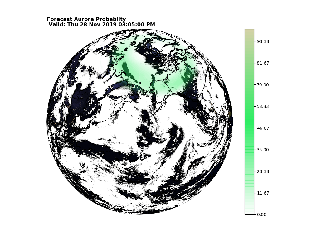
The end result of the tutorial will be an image that looks similar to this, but will be different depending on the time of day, auroral activity, and cloud cover:

Final Product: Forecast Aurora Probability and simulated GFS clouds valid UTC time.

Loading the background images

The first step is to download the "Blue Marble" and "Black Marble" background images to load into the dataset.  These are pretty easy to grab, I will simply provide links to the geotiff 0.1 degree versions for each image.  Load these into a folder where you can access them using a Python script.

• Blue Marble: Here
• Black Marble: Here

If these don't work you can try the parent sites: Blue Marble here, and Black Marble here.

Now that you have the data, it's time to load it into Python.  Before that however, the required packages for the entire tutorial need to be imported:

try:
    from urllib2 import urlopen
except ImportError:
    from urllib.request import urlopen

from io import StringIO

import numpy as np
from datetime import datetime, timedelta
import cartopy.crs as ccrs
from cartopy import feature as cfeature
import matplotlib.pyplot as plt
from matplotlib.colors import LinearSegmentedColormap 

from cartopy.feature.nightshade import Nightshade
from matplotlib.path import Path
from cartopy.mpl.patch import geos_to_path
import netCDF4 as NC

Note the"try" statement is used to make the script compatible with both Python 2.7 and Python 3 urllib syntax.  Now, once the data is imported, I'm going to define a common function to load the "Marble" images, since they have identical lat/lon boundaries.

def load_basemap(map_path):
    img=plt.imread(map_path)
    img_proj = ccrs.PlateCarree()
    img_extent = (-180, 180, -90, 90)
    return img, img_proj,img_extent

You should be able to see that the above function is really straightforward.  The image is first loaded into an array using "imread" from matplotlib, and then the image extent is set to span the entire glob (which is obvious from looking at the image), and then the image projection information for Cartopy is set to PlateCarree, since we are working in lat/lon coordinate space.  To investigate a little further, we can call this function and look at the shape of the image array.
Assuming the image is in the same folder as your script...

map_path='RenderData.tif'
bm_img,bm_proj,bm_extent=load_basemap(map_path)
print(np.shape(bm_img))

returns: (1800, 3600, 3)

Notice that the array returned has 3 dimensions despite the fact that it is a 2D image: the 3rd column is where the individual red/green/blue information for the image is stored, where as the first 2 columns correspond to the y and x pixels.  To demonstrate this, I'll plot each channel separately without geographic information.

plt.figure(figsize=(8,14))
ax=plt.subplot(311)
plt.pcolormesh(bm_img[:,:,0],cmap='Reds')
ax=plt.subplot(312)
plt.pcolormesh(bm_img[:,:,1],cmap='Greens')
ax=plt.subplot(313)
plt.pcolormesh(bm_img[:,:,2],cmap='Blues')
plt.show()

This produces the following image:

RGB channels for the Blue Marble image (Yikes! It's upside down!)

Note that where all three channels are saturated, the combined RGB image will be white (e.g., Antarctica), where as where all three channels are faded, the RGB image will appear back (e.g., the Oceans).  Also notice how the image is upside down, this will be addressed in the next part.

The question, is how can we plot the combined RGB image from the 3 dimensional array.  Instead of using the "pcolormesh" or the "contourf" functions, the "imshow" function is used.  this function, is versitile and naturally takes a 3D array assuming the 3rd axis (if there is one) is the RGB channel.  It also, takes the extent argument, which defines the image corners, without needed corresponding coordinate arrays.

    plt.figure(figsize=(11,8))
    ax=plt.subplot(111,projection=ccrs.PlateCarree())
    ax.imshow(bm_img,extent=bm_extent,transform=bm_proj,origin='upper')
    plt.show()

This results in the following image:

Blue Marble

I won't go into detail on how to load the black marble, however, I will provide the code used to load both images as they are read into the final product.

bm_img,bm_proj,bm_extent=load_basemap('RenderData.tif')
nt_img,nt_proj,nt_extent=load_basemap('BlackMarble_2016_01deg_geo.tif')

Blend Images using the Day/Night Delimiter

This next section is the crux of the whole tutorial: Basically, I'll explain how to use Cartopy Nightshade (Note: requires version 0.17 or higher) to mask out the day time blue marble and show the night time black marble image.  For this, I'll use the matplotlib "Path" function to draw a polygon "path" connecting the coordinate information associated with the Nightshade function.

The Nightshade function is a neat function that allows you to draw the day/night delimiter on a glob for a given datetime object.  In the full example, the datetime object will be defined by the aurora forecast, but for demonstration of Nightshade, the datetime.now() object will be used.

For a simple demonstration, simply copying the code to generate the blue marble image, with only a couple of added lines, provided you are following the tutorial with the package imports written as above:

plt.figure(figsize=(11,8))
ax=plt.subplot(111,projection=ccrs.PlateCarree())
ax.imshow(bm_img,extent=bm_extent,transform=bm_proj,origin='upper')
ax.add_feature(Nightshade(datetime.utcnow()),zorder=2,alpha=0.8,color='r')
plt.title(datetime.utcnow().strftime('%c'))
plt.show()

This will essentially mask out the "night sky" over the blue marble image, it's that simple!

Night masked out.

Now the goal here is simple: replace the "red" masked out section with the black marble image.  To do that, I'll first define a function to clip regions within the shapefile polygon.

The first step is to define the Nightshade "shape" from the Nightshade function:

nshade=Nightshade(datetime.utcnow())
transform=nshade.crs

Now we have both the nightshade shape, and the nightshade coordinate reference system, which is needed to ensure the projection transform is performed correctly.  From the shape, we grab the geometries (i.e., the polygons, or in this case ... polygon; singular).

geoms=list(nshade.geometries())

Here is the tricky part: because the Nightshade coordinate reference system is NOT Plate Carree (it's a rotated pole projection for those interested), it's important that the transform is done correctly.  If you assume the transform is Plate Carree you will end up with a mask that is wrong.  However, the matplotlib path function requires that the transform is a matplotlib transform, and not a cartopy crs object.  So, to do this conversion, I will define a "dummy" transform when defining my Caropy subplot that equals the crs from the nightshade object.

fig = plt.figure(figsize=(10, 8))
ax = fig.add_subplot(1, 1, 1, projection=ccrs.PlateCarree(),transform=nshade.crs)

Now, we have a defined figure, and a matplotlib transform that matchs the nightshade object, we're ready to mask.  First we plot the blue and black marble images on the same subplot, and then use the geos_to_path and Path functions imported at the top of the script:

plt.figure(figsize=(11,8))
ax=plt.subplot(111,projection=ccrs.PlateCarree(),transform=nshade.crs)
im0=ax.imshow(bm_img,extent=bm_extent,transform=bm_proj,origin='upper',zorder=1) 
im1=ax.imshow(nt_img,extent=nt_extent,transform=nt_proj,origin='upper',zorder=2)
path = Path.make_compound_path(*geos_to_path(geoms))
im1.set_clip_path(path, transform=ax.get_transform())
plt.title(datetime.utcnow().strftime('%c'))
plt.show()

And the blended image is complete,note that the subplot transform is used in the set_clip_to_path function:

Blended image based on current datetime.

Now, it's time to plot the aurora forecast.

Loading and Plotting the Aurora Forecast

This section will mostly be a reproduction of the code demonstrated here, with some minor differences.  Esentially, Numpy loadtxt is used to load the ascii data from the SWPC into a 2 dimensional array and the array is plotted on the map.  The first step is to define a cool looking aurora color bar.  This a a direct reproduction from the Cartopy example because I think they did a nice job with the color scales.

def aurora_cmap():
    """Return a colormap with aurora like colors"""
    stops = {'red': [(0.00, 0.1725, 0.1725),
                     (0.50, 0.1725, 0.1725),
                     (1.00, 0.8353, 0.8353)],

             'green': [(0.00, 0.9294, 0.9294),
                       (0.50, 0.9294, 0.9294),
                       (1.00, 0.8235, 0.8235)],

             'blue': [(0.00, 0.3843, 0.3843),
                      (0.50, 0.3843, 0.3843),
                      (1.00, 0.6549, 0.6549)],

             'alpha': [(0.00, 0.0, 0.0),
                       (0.70, 1.0, 1.0),
                       (1.00, 1.0, 1.0)]}

    return LinearSegmentedColormap('aurora', stops)

Basically, a dictionary with 0-1 values for red (r), green (g), blue (b), and transparancy (alpha) is passed to the LinearSegmentedColormap function which defines a color map that basically linearly interpolates between each of the 9 "stops" defined by the user.

Now, that the colormap is defined, you can pull the aurora data from the SWPC and load it into an array:

    # To plot the current forecast instead, uncomment the following line
    url = 'http://services.swpc.noaa.gov/text/aurora-nowcast-map.txt'

    response_text = StringIO(urlopen(url).read().decode('utf-8'))
    aurora_prob = np.loadtxt(response_text)
    # Read forecast date and time
    response_text.seek(0)
    for line in response_text:
        if line.startswith('Product Valid At:', 2):
            dt = datetime.strptime(line[-17:-1], '%Y-%m-%d %H:%M')

Now, again this code is largely copied from the Cartopy example, but essentially you're reading the text information from the URL, first into the Numpy loadtxt function, which is a natural fit for this data, since the function, by default, assumes "#" is a comment, and "spaces" are delimiters, so in this instance, no additional arguments are required for loadtxt.  Then, the datetime associated with forecast is read into a datetime object.

Since it is known that the lat/lon data spans -90 to 90 and -180 to 180, we define lat/lon arrays based on the shape of the aurora data:

lons=np.linspace(-180,180,np.shape(aurora_prob)[1])
lats=np.linspace(-90,90,np.shape(aurora_prob)[0])

Finally, combining everything together to product the "cloud-free" aurora forecast:

plt.figure(figsize=(11,8))
ax=plt.subplot(111,projection=ccrs.PlateCarree(),transform=nshade.crs)
im0=ax.imshow(bm_img,extent=bm_extent,transform=bm_proj,origin='upper',zorder=1)
im1=ax.imshow(nt_img,extent=nt_extent,transform=nt_proj,origin='upper',zorder=2)
path = Path.make_compound_path(*geos_to_path(geoms))
im1.set_clip_path(path,transform=ax.get_transform())   
Z=ax.contourf(lons,lats,np.ma.masked_less(aurora_prob,1), levels=np.linspace(0,100,61), transform=ccrs.PlateCarree(),     zorder=5,cmap=aurora_cmap(),antialiased=True)
plt.title(datetime.utcnow().strftime('%c'))
plt.show()

Which gives you the following image:

Aurora Forecast with Plate Carree Projection

Finally, replacing the PlateCarree map projection with the NearsidePerspective projection, we get something a little bit closer to the final image:

fig = plt.figure(figsize=[10, 8])
ax = plt.axes(projection=ccrs.NearsidePerspective(-170, 45),transform=nshade.crs)
im0=ax.imshow(bm_img,extent=bm_extent,transform=bm_proj,origin='upper',zorder=1)
im1=ax.imshow(nt_img,extent=nt_extent,transform=nt_proj,origin='upper',zorder=2)
path = Path.make_compound_path(*geos_to_path(geoms))
im1.set_clip_path(path, transform=ax.get_transform())
Z=ax.contourf(lons,lats,np.ma.masked_less(aurora_prob,1), levels=np.linspace(0,100,61), transform=ccrs.PlateCarree(),

              zorder=5,cmap=aurora_cmap(),antialiased=True)
plt.title("Forecast Aurora Probabilty \n Valid: %s"%dt.strftime('%b/%d/%Y %H:%M UTC'),

          loc='left',fontweight='bold')

Orthographic / Nearside Perspective Projection

Adding A Cloud Forecast from the GFS

The final step in this tutorial is to add cloud cover from the GFS to the map.  This is unnecessary, if you're happy with the above image, but my personal thought is, you aren't going to see the aurora if it's cloudy, so having the forecast cloud cover is a nice overlay.  It's real easy to add the clouds, simply pull the GFS data from the NOMADS server using netCDF4, match the GFS model time to the aurora forecast time and overlay the total cloud cover variable on the map.  Again, my assumption is that if you've made it this far, you're comfortable working with GFS data using netCDF4 and I won't explain in detail why the following code works:

dhour='12' ## or 00, or 18 or 06, your choice
dtstr=dt.strftime('%Y%m%d')
gfs_path='http://nomads.ncep.noaa.gov:80/dods/gfs_0p25_1hr/gfs%s/gfs_0p25_1hr_%sz'%(dtstr,dhour)

gfs_data=NC.Dataset(gfs_path,'r')

gfslons=gfs_data.variables['lon']
gfslats=gfs_data.variables['lat']

tres=gfs_data.variables['time'].resolution
tmin=datetime.strptime(gfs_data.variables['time'].minimum,'%Hz%d%b%Y')
times=[timedelta(hours=float(i)*24.*tres)+tmin for i in range(len(gfs_data.variables['time'][:]))]

tidx=np.argmin(np.abs(np.array(times)-dt))

clouds=gfs_data.variables['tcdcclm'][tidx,:]

and then simply add the following code to the beneath the code used to load the background images and plot the aurora forecast:

ax.pcolormesh(gfslons[:],gfslats[:],np.ma.masked_less(clouds,75.),transform=ccrs.PlateCarree(),
    alpha=0.7,cmap='Greys_r',zorder=4,vmin=50,vmax=100)

And voila:

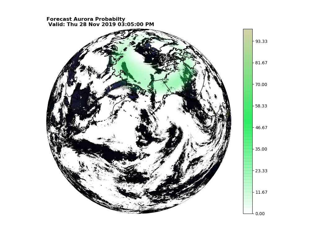
Final Product

Final Notes

That is all for this tutorial, it was a long one, but I think there is a lot of useful stuff in here.  A few final notes, reprojecting the background images can lead to really poor quality images, I find this particularly true for Lambert and PolarStereo projections, so be aware of that. 

Read More

Tutorial: The difference between self describing and non-self describing NETCDF files, and how to write them

In writing posts for this blog, I try my best to avoid what could be considered "mission creep," or writing coding tutorials that at best only tangentially related to GrADS.  This tutorial is verging upon what could be considered mission creep and has as much to do with teaching "good data" practices as it does with teaching GrADS skills.  Furthermore, there are no GrADS scripting lessons to be learned here, and the only code I provide is written for Python. 

All that said, in this tutorial, I will be showing you how to write NETCDF files that can be read using GrADS using both the self describing 'sdfopen' and non-self describing 'xdfopen' commands. I do this because, you may one day find yourself with some gridded data set that you want to plot using GrADS, however this data set may be in a text file format, or perhaps maybe you need to perform higher level calculations on the data that cannot be performed in GrADS before you display it.  While you could write the data out as a binary data file with a GrADS control file, maybe you are more comfortable with the NETCDF format (I know I certainly am).  Plus there are other benefits to using NETCDF instead of binary; one example is cross compatibility. NETCDF files can be read in with pretty much any data analysis software, so not only can you read your file in GrADS, but you can read it in with Matlab, IDL, R, Python, etc., as well.

What makes a NETCDF file self describing?

It's all about the metadata!  Metadata is often referred to "data about the data."  For example, metadata includes things like:

• The data and time a file was created
• What data is in the file
• Units of variables within the file
• Information about the coordinates (e.g., lat, lon vs. x,y)
• If the data file is for model output it might include information such as 

• Resolution, parameterizations, time step

Metadata is super important, and learning how to include it in any data set you are producing/sharing is a critical skill in a scientific career.  We are lucky in meteorology because there have been solid efforts to standardize metadata practices in the past couple of decades.  Now, NETCDF makes it very easy to provide good metadata, so there is no excuse not to do it.  So if nothing else, I hope to get that point across to you with this tutorial.  To really drive this point home, here is a meme.

 

To make a file self-describing (that is such that GrADS can read the file in with NO accompanying control file required using the 'sfdopen' command) the metadata including in the NETCDF file must adhere to the COARDS data standards: More information on COARDS here.  Personally, I didn't find this website all that useful when figuring out how to make self-describing NETCDF files, but it does provide some nice background.

How to write a self describing NETCDF file (SDFOPEN)

Here I will provide the key metadata required to write a self-describing NETCDF file.  The example, I provide is sub-setting the first 24 hours of GFS temperature data from the 00z December 30th 2015 run.  If you choose to try and reproduce these results, you will need to update the date.  I will us python to read in the data from the GrADS Data Server (GDS) and to write the local NETCDF file.  You could use any program of your choice to do this, so long as it reads and writes NETCDF files.  The python script is included in this tutorial.

So the most important thing to understand when writing your datafile is that your coordinate dimensions and accompanying dimension variables (e.g., lat,lon) adhere to the COARDS guidelines, otherwise GrADS will not open your file.  For example, you might get an error like:

     gadsdf: SDF file has no discernable Y coordinate

The metadata for the non-dimension variables (e.g., temperature, u,v) is more up to the person writing the file.

Assuming you know how to read in the NETCDF file and data from the GDS, in python:

   datafile='http://nomads.ncep.noaa.gov:9090/dods/gfs_0p25/gfs20151230/gfs_0p25_00z'
   cdata=netCDF4.Dataset(datafile,'r')
 
To start writing the file, we will first look at the dimensions and dimension variables.
You must include the following dimensions and variables in your NETCDF file:

• lat
• lon
• time
• lev

 In python you will make these dimensions and variables as such:

   newdata=netCDF4.Dataset(newfile,'w')
   newdata.createDimension('lat', len(lat[lmin:lmax]))
   newdata.createDimension('lon', len(lon[lomin:lomax]))
   newdata.createDimension('lev', len(lev[:]))
   newdata.createDimension('time', 8)

Where lmin,lmax,lomin,lomax are indices that mark your subset boundaries.
Then in addition to creating the dimensions, you must make the variables as well (For example latitude):

   latvar=newdata.createVariable('lat','f8',('lat'))

Now you need to populate latvar with metadata.  To determine what metadata you need, I simply printed out the 'lat' variable from within the GDS datafile as this datafile is self-describing and adheres to the COARDS standards.  If you've seen my other tutorials I often access these files using the 'sdfopen' command.  In doing that, I get the following (again this will look different if you aren't using python):

<type 'netCDF4.Variable'>
float64 lat(lat)
    grads_dim: y
    grads_mapping: linear
    grads_size: 721
    units: degrees_north
    long_name: latitude
    minimum: -90.0
    maximum: 90.0
    resolution: 0.25
unlimited dimensions:
current shape = (721,)

These are the metadata that you need to include for the latitude variable in your NETCDF file.  The dimensions will change, because you are sub setting the data, but things like 'grads_dim' and 'grads_mapping' need to be the same.  In python adding metadata to a NETCDF variable is easy:

   latvar.grads_dim='y'
   latvar.grads_mapping='linear'
   latvar.grads_size=str(len(lat[lmin:lmax]))
   latvar.units='degrees_north'
   latvar.long_name='latitude'
   latvar.minimum=str(lat[lmin])
   latvar.maximum=str(lat[lmax])
   latvar.resolution='0.25'
   latvar[:]=lat[lmin:lmax]

Again, remember with the sub setting, the lmin and lmax indices are required to match the output file.
Now if I print out MY latitude variable within the output NETCDF file it looks similar to the GDS file with only minor differences:

<type 'netCDF4.Variable'>
float64 lat(lat)
    grads_dim: y
    grads_mapping: linear
    grads_size: 200
    units: degrees_north
    long_name: latitude
    minimum: 10.0
    maximum: 60.0
    resolution: 0.25
unlimited dimensions:
current shape = (200,)

You will need to do the same thing for the other dimension variables (lon,lev,time) with a few minor differences.  I don't explicitly show the steps here to save space and redundancy.  You can find the steps written down in the accompanying .py file.

Once you have your dimension variables, you need to add the temperature variables.  In the example, I have you add both the 2 meter temperature and the temperature as a function of pressure level.  This is to show you how to add variables with differing dimensions.

As I stated earlier, there are fewer restrictions for these variables than the dimension ones.  But it is still a good practice to add metadata.  When printing out the GDS 'tmp2m' var, you get this:

<type 'netCDF4.Variable'>
float32 tmp2m(time, lat, lon)
    _FillValue: 9.999e+20
    missing_value: 9.999e+20
    long_name: ** 2 m above ground temperature [k]
unlimited dimensions:
current shape = (81, 721, 1440)

So for our variable, we will try to match this as close as possible:
  gtmpvar=newdata.createVariable('GTMP','f4',('time','lat','lon'),fill_value=9.999E20)
  gtmpvar.long_name='2 Meter Temperature'
  gtmpvar.units='K'
  gtmpvar[:]=var1[:8,lmin:lmax,lomin:lomax] ## Add the actual data from the GDS file

And that's it for the 2 meter temperature.  Now, you can do the exact same thing for the vertically varying temperature with only minor changes:
   tmpvar=newdata.createVariable('TEMP','f4',('time','lev','lat','lon'),fill_value=9.999E20)
   tmpvar.long_name='Pressure Interpolated Temperature'
   tmpvar.units='K'
   tmpvar[:]=var2[:8,:,lmin:lmax,lomin:lomax]

The big difference here, is that in the dimensions section of the createVariable function includes a dimension for 'lev'.

When you are done, close out your file and you can then open it in GrADS using the 'sdfopen' command.  Then if you display the temperature data, you should get something that looks like this:

How to read and write a NON self describing NETCDF file (xdfopen)

If you want to read a file that is not self-describing into GrADS, you need to include a control file.
Essentially, you need to treat the NETCDF file as if it were a binary data file.

Now for this tutorial, we will run through the exact same process, highlighting the differences in how we write metadata to the NETCDF file.

Starting with the dimension variables, we will no longer include the metadata that we did for the self describing file:

    newdata=netCDF4.Dataset(xdffile,'w')
    newdata.createDimension('lat', len(lat[lmin:lmax]))
    latvar=newdata.createVariable('lat','f8',('lat'))
    latvar[:]=lat[lmin:lmax]

Similarly, I'll skip the rest of the dimension variables, but as you see, all I did was define the variable and add the data to it.  For simplicity, and since it doesn't matter, I'll keep the temperature variables as they were in the self describing example.

Now the NETCDF file is created.  If however you try to open this file using the 'sdfopen' command, you will get an error.  So we need to create a control file.

The control file can be easily written using python (as in this example) or whatever program you are using.  I'm going to copy the code to write the control file below, and explain it after.

    ### Now write the control file ###
    xdfctl='C:/OpenGrADS/xdffile.ctl'
    xdflocal='xdffile.nc'
    xdf = open(xdfctl, 'w')
    xdf.write('DSET ^' + xdflocal +'\n')
    xdf.write('TITLE XDF example File 00z30dec2015 \n')
    xdf.write('UNDEF 99999.0\n')
    xdf.write('XDEF lon '+str(len(lon[lomin:lomax]))+' LINEAR ' + str(lon[lomin]) +' 0.25\n')
    xdf.write('YDEF lat '+str(len(lat[lmin:lmax]))+' LINEAR ' + str(lat[lmin]) +' 0.25\n')
    xdf.write('ZDEF lev '+str(len(lev[:]))+' LEVELS ')
    for i in lev[:]:
        xdf.write(str(int(i))+' ')
    xdf.write('\n')
    xdf.write('TDEF time 8 LINEAR 00z30dec2015 3hr\n')
    xdf.write('VARS 2\n')
    xdf.write('GTMP=>GTMP 0 99 2-meter Temperature [k]\n')
    xdf.write('TEMP=>GTMP '+str(len(lev[:]))+' 99 Temperature [K]\n')
    xdf.write('ENDVARS')
    xdf.close()

The most important take away to learn about writing a control for a NETCDF file is that you match the variable/dimension names in the control file to the variable/dimension names in the NETCDF file (case sensitive).

For example: 'GTMP=>GTMP' will only work if there is a variable in the NETCDF file called 'GTMP'.  Similarly, following the XDEF definition, you need to point to the longitude variable (lon) in the NETCDF file.  This is different than writing out control files for binary datasets which don't require anything after XDEF.

Other than that, you see some other things, the levels are defined in a special way since the vertical coordinate is not incremented linearly.  Also the lat/lon sizes are not hard coded, to allow you to make bigger or smaller spatial subsets without a lot of extra work.

Open the control file in GrADS using the 'xdfopen' command:

'xdfopen xdffile.ctl'

A few notes on using the control file:

Note that the coordinate data is not actually read
from the NETCDF file, it is inferred from the control file.  So it is important that the resolution and the starting points are right, otherwise you will get an incorrect result, even if your longitude data is correct in the NETCDF file.  For example, comparing the correct (0.25) resolution to an incorrect resolution (0.45) gives the two different maps shown on the right.  So get the resolution right!

One final note: This kind of control file only seems to work with nice rectangular datasets.  That is lat/lon coordinates that vary independently from one another.  If your lat/lon grid does not vary independently (i.e., longitude is a function of y and visa-versa), then using this method will warp tour map projection.  In these situations it is recommended that you write your data out to a binary file with the PDEF option.  I have yet to get the PDEF option to work with a NETCDF file.






So that is it for the tutorial, hopefully you have a better understanding regarding the difference between self describing and non self describing NETCDF files, and how to write and open them in GrADS.  No GrADS scripts to download here, but a full python script (version 2.7) is included that will reproduce the files and plots generated in this tutorial.  You will need the netCDF4 module installed for this script to work however.  Numpy and sys are standard I believe.  Also you may need to update the date.

Download Python Script here

Read More

Tutorial: GrADS Widgets, and GUI capabilities; Make a functional calculator using GrADS

This tutorial will show you how to use a few of the widgets that come with GrADS to create basic Graphical User Interfaces (GUIs).  We will use these tools, to create a functional calculator.  This exercise should familiarize you with how to make basic GUIs using the GrADS scripting language.

I have been on the fence about writing a full tutorial about GrADS widgets, as there is already a lot of good material out there describing how to use them.  Though ultimately I decided that it would be beneficial to have a more in depth tutorial that really details some of the logic involved.  So, if you are just looking for fast reference, this tutorial may be a bit much.  If you are looking for a quick reference, I encourage you to check out this site.

Before you start the tutorial, you may be thinking to yourself; "Why go through all the effort to write GUIs?"  GUIs are nice because they are what most people are familiar with, and often times I find it easier to use a GUI interface that has many preset options built in, rather than slightly editing code, or manually inputting different values into the console.  So in that respect, it is worth the upfront time and effort to write the GUI, so you can accomplish a wide variety of operations with the click of a button.

Lets get started, as always (and so you know what the end goal is), below is an image of the finished product.

Calculator GUI

In writing this tutorial, I have wracked my brain a little trying to figure out a nice way to summarize GUI structure using the GrADS widgets.  The best thing I could come up with is that when you write a GUI, you need to create the infrastructure first; the buttons, the drop menus, etc., then you need to write the functions of each individual component of that infrastructure.

The first thing we need to do is set up the infrastructure of the GUI, this will serve as sort of the skeleton that the calculator functions will work with.

To set up the GUI infrastructure, we are going to break the buttons into 4 groups.

1. Number Keys
2. Basic Operators (+ - * /)
3. Special Operators (sin/cos/etc.)
4. Other (Quit, Ce, Enter)

In addition to the GUI components, we need to include some dynamic updating of the "Display Screen."  This will be straightforward though, as we will just use the 'draw recf' and 'draw rec' commands to update the display.  Before we get to the display, we will start by going through writing each group of widgets separately.

Group 1: The Number Keys:

Since this is the first examination of the GrADS 'Button' widget, I will briefly explain the syntax used.  So the two relevant commands for the Button widget are: 'set button', 'draw button' and 'redraw button.'  The first two commands are followed by numerous arguments, the last one only requires one argument, and determines if the button is in the "on" or "off" position.

The "set button" command sets up the style of your button, the color, the text color, and the borders.

'set button' takes up to 9 arguments taking the form of:

'set button 1 15 1 1 2 15 1 1 3'

Where the first 4 arguments represent the OFF position; text color, face color, bright color for border shading, and the dark color for the border shading.  The second 4 arguments represent the same thing, but for the ON position.  The Final argument, sets the thickness of  your shaded border, with large numbers creating a noticeable 3D bevel effect, and small values basically draw a line around your button.  The above command is the style used for the calculator,  and it sets the number key buttons to be gray colored with white text when off, and gray colored with red text when on.  A few other examples are shown below.

• button1:   'set button 1 4 6 7 1 2 7 6 30'
• button2:  'set button 5 8 15 1 5 8 15 1 30'
• button3:  'set button 2 3 15 1 2 3 15 1 1'

Button Examples

Now that we have covered the 'set button' command, we need to look at the 'draw button' command.

The "draw button" command requires 6 arguments or it will send back an error.  The arguments are as follows:

1. Identifying Number
2. center in x (page coordinates)
3. center in y (page coordinates)
4. width
5. height
6. string

The most important argument is the Identifying number.  This number is how you tell this button apart from all the other buttons in the GUI.  It is important that you ensure that your buttons number is unique so that you don't have weird things happen when you click on it.  Beyond that, the remaining arguments are just for formatting purposes, setting the button boundaries as well as the string (what the user sees).

Example: 'draw button 1 5.5 5.5 1 1 Button1'
This would draw a square button, labeled Button1 in roughly the center of the GrADS display.

Now that we are familiar with the 'set button' and 'draw button' commands, we can see how to write out the number keys of our calculator.

I like to do everything inside of a loop.  Generally, if I need to execute a command more than once, I try to use a loop to reduce the amount of text I actually have to write, so that's what we are going to do here.  We are going to loop through each number 1-9, draw each row of buttons, and then draw the remaining two buttons (0 and .) on the last row.  Since this is an advanced tutorial, I will just copy down the code for the loop, and let you make sense of it.

  *Environmental Variables to set scale*
  cols=3
  nums=11
  bnum=1
  w=0.75
  xstart=3.5
  ystart=5.5
 ****

   'set button 1 15 1 1 2 15 1 1 3'
   y=ystart
  while(bnum<=nums)
    col=1
    x=xstart
    while(col<=cols)

      if(bnum<=9)
        'draw button 'bnum' 'x' 'y' 'w' 'w' 'bnum
      else
        if(bnum=10);'draw button 'bnum' 'x' 'y' 'w' 'w' 0';endif
        if(bnum=11);'draw button 'bnum' 'x' 'y' 'w' 'w' .';endif
      endif

      x=x+w*1.5
      col=col+1
      bnum=bnum+1
    endwhile
    y=y-w*1.5
  endwhile

This code, will draw all 11 buttons (0-9, and the decimal point).  The environmental variables are there so you can play with the size and shape.  Just make sure you note that each button is given its own unique identifying number, that number will come in handy later when we set up the actual functions associated with each button.  The fact that each identifying number is equal to the string also comes in handy later.

Group 2: The Basic Operators:

This code is similar the code used to write the number keys, but with minor differences.  Once again, we use a loop to write out the operators.

  cols=2
  strings='+ - * /'
  bnum=12
  nums=16
  xstart1=x
  y=ystart

  'set button 0 4 15 1 2 4 15 1'

  while(bnum<nums)
    col=1
    x=xstart1
    while(col<=cols)
      str=subwrd(strings,bnum-11)
      'draw button 'bnum' 'x' 'y' 'w' 'w' 'str
      x=x+w*1.5
      col=col+1
      bnum=bnum+1
    endwhile
    y=y-w*1.5
  endwhile  

A few important things to notice in the above code:

• We use the 'set button' command to reset the button to have a blue face
• We change the number of columns to 2
• We use a master string that has all 4 sub-strings representing each operator
• See: Tutorial on Arrays if you are unfamiliar with this
• We start the identification number (bnum) at 12 so that it doesn't interfere with the buttons already created

Group 3: Special Operators

In order to illustrate the use of the 'drop menu' I chose to include a few "special" math functions in the calculator that you would access using a nested drop menu.  So the drop menu syntax in GrADS is a little different than the 'draw button' syntax.

Similar to the button widget, the drop menu also has a formatting precursor 'set dropmenu'  This command takes up to 15 arguments, corresponding to different formatting options like text color, borders, widget color.,etc.  These 15 arguments are well described here and in the interest of time, will not be thoroughly discussed in this tutorial.  Though similar to 'set button' these values correspond to the same attributes, but under different circumstances, e.g., whether or not a given option is selected.  I'll be honest, I usually just ignore the 'set dropmenu' command and use the default options, but you could make a really slick interface with fully customized colors and borders using this command if you so chose.

The 'draw dropmenu' command is fairly straightforward.  Similar to 'draw button' it requires 6 arguments, and the first 5 are identical to the first 5 arguments for 'draw button'.  Again, be sure that your drop menus identification number is unique. The last argument is your drop menu.  It is a collection of strings that represent different options with each option separated by a "|"

Example: 'draw dropmenu 1 5.5 5.5 1.1 0.7 Menu | option1 | option2 | option3'

The string before the first "|" is what the user sees on the display when the dropmenu is not selected.

Drop menus can be nested or "cascaded" with a small addition to the string at the end of the menu.  Using the above example we can get a cascading menu from option 3 by altering it as such:

'draw dropmenu 1 5.5 5.5 1.1 0.7 Menu | option1 | option2 | option3 >10> '

This now tells your widget that you want option3 to point to a cascading drop menu with the identification number 10.  Now, we just need to set up that cascading menu.  For this, we use the 'draw dropmenu' command again, except we replace all of the spatial variables with the word "cascade."  This specifies that you want this menu to be attached to another menu.  Then, the syntax is the same, you need the identification number (in our example 10) followed by your options.

'draw dropmenu 10 cascade cascade1 | cascade2 | cascade3 '

So that it is for the basics behind the drop menu and the cascading (nested) drop menus.
Now that we know how to use the 'draw dropmenu' command, I will show you how it's used in our calculator!  This is actually easy, since we only have one drop menu in the calculator.

  x=xstart1+w*0.75
  h=w
  w=2*(w)+w*0.5

  'draw dropmenu 16 'x' 'y' 'w' 'h' Special | e^x | x^2 | ln(x) | Trig >03> '
  'draw dropmenu 3 cascade sin(x) | cos(x) | tan(x) '
  
First we simply reset the location and size of the drop menu relative to the rest of the calculator, then we just draw the drop menu.  Notice that the parent drop menu has a unique identifying number, but the nested menu does not.  This is because the identification for the cascading menu is in a different spot than the identification for the parent, so this does not need to be unique (More on this soon).


Group 4: Other

The last group, the other important buttons; Enter, Clear (CE) and Exit and the display.  The exit button is important as it will break the loop within the GUI, more on this when we build in the GUI functionality.  But since there is nothing particularly new here, I'll just give you the code, and you should be able to see what it is doing.

Starting with the Display:

recxlo=xstart-w*0.5
recylo=ystart+0.75
recxhi=xstart+w*4.5
recyhi=ystart+1.75

'set line 1 1 1'
'draw recf 'recxlo' 'recylo' 'recxhi' 'recyhi

'set line 15 2 6'
'draw rec 'recxlo' 'recylo' 'recxhi' 'recyhi

The display just draws a couple of rectangles above the button interface.

Then the Buttons:

ymid=(recyhi+recylo)/2
xmid=recxhi+0.75
y=y-h*1.5

'draw button 100 'xmid' 'ymid' 'w*1.25' 'w*1.25' CE'
'draw button 101 'recxlo+w*0.625' 'y-1.25' 'w*1.25' 'h' Quit'
'draw button 102 'recxlo+w*2.20' 'y-1.25' 'w*1.25' 'h' Enter'

And that should draw out the full calculator!  If you haven't done so already, now may be a good time to take a quick break.  Below we move away from building the infrastructure and get into designing the functionality to our calculator.

The entire functionality of the GUI interface is based on the 'q pos' command.  This command prompts the user to click somewhere on the display screen and returns information including the page coordinates, mouse button, and widget properties.  More details on the 'q pos' command can be found here.

The basic design we will use is a loop that keeps prompting the user to click on the screen until the 'quit' button is pressed.  Within the loop is where the magic happens.  So we first set up the loop, with the condition for exiting.  Before we start the loop, we need to set up a few initial conditions.  Since the calculator performs math operations on two numbers, we will need two numbers for variables, and a variable for the returned number. Lastly, we need a variable that represents the operator.  So we do that before the loop.

  calculated=0
  num1=''
  num2=''
  op=''

  while (1)
    'q pos'
    num = subwrd(result,7)
    if (num=101); break; endif;

This sets up the initial conditions and starts the loop, and gathers the information about which button you are pressing using the 'subwrd()' function. Remember, the 'Quit' button identifier is 101, so we set the condition that if the returned button is 101, we break the loop.

Now, lets write down the code that sets up the numbers.  I'm going to just show the code, and explain it after.

  if(num !=-1 & num!=16 & num!='')

    'redraw button 100 0'
    'redraw button 101 0'
    'redraw button 102 0'

    if(num<12)

      if(num<10);out=num;endif
      if(num=10);out=0;endif
      if(num=11);out='.';endif

      if(op='')

        num1=num1''out
        'set line 1 1 1'
        'draw recf 'recxlo' 'recylo' 'recxhi' 'recyhi
        'set line 15 2 6'
        'draw rec 'recxlo' 'recylo' 'recxhi' 'recyhi
        'draw string 'recxhi-0.25' 'ymid' 'num1
      endif

      if(op!='')

        num2=num2''out
        'set line 1 1 1'
        'draw recf 'recxlo' 'recylo' 'recxhi' 'recyhi
        'set line 15 2 6'
        'draw rec 'recxlo' 'recylo' 'recxhi' 'recyhi
        'draw string 'recxhi-0.25' 'ymid' 'num2

      endif
    endif

We start first with the condition that num is equal to something, and something other than the dropmenu.  This sets it so that you can click all over the screen as many times as you want and nothing will happen.  We then reset all of our miscellaneous buttons to the off position (this is purely for formatting, the actual button status is not used in any of the functions).

To get the functionality of the buttons, we start by checking the condition that the num<12.  This checks whether or not you are adding a number, or doing something else.  Within that condition, there is the check for whether or not there is an operator set.  Since we want to make this like a real calculator, if an operator is set, we put our numbers into num2, and if it isn't we put it into num1.  We set numbers by concatenating strings, so you just keep pressing numbers to build up your number.  We also need to distinguish if we add a number, or a 0 or a decimal point.  Once our number is changed, we wipe the display and redraw it with the chosen number.  This happens so fast, that it appears as if you are just entering numbers into the calculator.

Next, we need to set up the operators.  To keep things simple, and since there is already a conditional statement isolating the drop menu, we'll first stick with the first basic operators.

    if(num=12);op='+';endif
    if(num=13);op='-';endif
    if(num=14);op='*';endif
    if(num=15);op='/';endif


    if(num>=12 & num<=15)
      bcount=1
      buttons=11
      while(bcount<=buttons)
        'redraw button 'bcount' 0'
        bcount=bcount+1
      endwhile
    endif

This code just uses a bank of conditional statements to set the operator up.  Once the operator is set up, and as long as you have selected a basic math operator the program loops through and sets all numbered buttons to the off position.  Next up, the special operators.  Note: This code is a little out of position, since the code that makes the calculations is within the conditional that excludes num=16.  But it seemed to make more sense in this order for the tutorial.

  if(num=16)
    special=subwrd(result,8)
    if(special=4)
      special=subwrd(result,10)+10
    endif

    if(special=1);op='exp';endif
    if(special=2);op='pow';endif
    if(special=3);op='ln';endif

    if(special=11);op='sin';endif
    if(special=12);op='cos';endif
    if(special=13);op='tan';endif

    'set line 1 1 1'
    'draw recf 'recxlo' 'recylo' 'recxhi' 'recyhi
    'set line 15 2 6'
    'draw rec 'recxlo' 'recylo' 'recxhi' 'recyhi
    'draw string 'recxhi-0.25' 'ymid' 'op'('num1')'

  endif

Since the drop menu identifier is in a different location when 'q pos' is called, we need get the drop menu identifier first.  We then need to check if the drop menu is equal to the cascade, in which case, we need to get the cascade option.  I add 10 to easily differentiate from the other values.  Then, we just set the op to the special values, and display the operator on the screen.

Finally, we are almost done.  Now we have all of our information, and we are ready to calculate our numbers!  Going back into the conditional statement that excludes num=16.  We start with the conditional value of 102 (the 'Enter') button.

    if(num=102)
      if(op!='')
        if(num1='');num1=0;endif
        if(op='+');calculated=num1+num2;endif
        if(op='-');calculated=num1-num2;endif
        if(op='*');calculated=num1*num2;endif
        if(op='/');calculated=num1/num2;endif


***     ***SPECIAL OPERATIONS****

        if(op='exp');calculated=math_exp(num1);endif
        if(op='pow');calculated=math_pow(num1,2);endif
        if(op='ln');calculated=math_log(num1);endif

        if(op='sin');calculated=math_sin(num1);endif
        if(op='cos');calculated=math_cos(num1);endif
        if(op='tan');calculated=math_tan(num1);endif

        num1=calculated
        num2=''

       'set string 0 r 6'
       'set strsiz 0.2
       'set line 1 1 1'
       'draw recf 'recxlo' 'recylo' 'recxhi' 'recyhi
       'set line 15 2 6'
       'draw rec 'recxlo' 'recylo' 'recxhi' 'recyhi
       'draw string 'recxhi-0.25' 'ymid' 'calculated

        op=''
        bcount=1
        buttons=12
        while(bcount<=buttons)
          'redraw button 'bcount' 0'
          bcount=bcount+1
        endwhile

        bcount=12
        buttons=16
        while(bcount<=buttons)
          'redraw button 'bcount' 0'
          bcount=bcount+1
        endwhile

      endif
    endif

This code looks long, but it's more of the same.  The only thing new is the block of conditional statements that performs the calculations based on what operation you have in place.  Then you set num1 to the calculated value, so you can continue to make calculations using the newly calculated number.

Now, we have one last loose end to tie up before we are finished with the calculator.  The 'Ce' button.
This button is designed to reset all the initial conditions, and redraw the display.

    if(num=100)
     num1=''
     num2=''
     op=''
     calculated=0

     'set line 1 1 1'
     'draw recf 'recxlo' 'recylo' 'recxhi' 'recyhi
     'set line 15 2 6'
     'draw rec 'recxlo' 'recylo' 'recxhi' 'recyhi
     'draw string 'recxhi-0.25' 'ymid' 0'
    endif
 endwhile

That about does it!  You now have a working calculator!  More importantly, you should have a pretty good foundation in creating GUIs in GrADS using the 'button' and 'drop menu' widgets.  If you followed the code segments throughout the script, it may be difficult to get a working script together due to some of it being out of order.  It is therefore recommended that you download the script provided, and edit that as you please.

I recommend that you play around with this script, change button styles, add or subtract special functions, etc.  I hope you enjoyed this tutorial, and hopefully you learned something about using GrADS widgets.  As always, feedback is much appreciated.


Download Example Script Here 

Read More