Tutorial: Use basemap.gs to make a beautiful map of "SST", Sea Ice and Snow in GrADS

This tutorial will draw upon many of the skills discussed in several other tutorials on this site, e.g., how to handle multiple files at once, or how to use basemap.gs.  There isn't too much "new" information in this tutorial on how to use these different features and functions of GrADS, rather this tutorial will show you how to specifically make a very pretty map of sea-surface temperature, sea ice, and snow.  The final outcome is shown below.

For this tutorial you will need:

• color.gs 
• xcbar.gs
• colormaps.gs
• basemap.gs (plus the accompanying .asc files)

Snow Cover and Sea Ice on the Robinson Map Projection

So before we start, I want to give a full disclaimer: The plot is not actually showing any observed SST.  In this tutorial I'm going to use the 0.25 degree GFS surface temperature.  In practice the surface temperature should be roughly equal to the SST over the Oceans.

The first thing we need to do is open both the GFS data and the sea ice data.  This data will come from NOMADS and will be opened using the 'sdfopen' command.  Note, the files below are for February 2015, so keep in mind, that you will need to change the date on files if you wish to copy paste the example code below.


   'reinit'
   gfsfile='http://nomads.ncep.noaa.gov:9090/dods/gfs_0p25/gfs20150218/gfs_0p25_18z'
   icefile='http://nomads.ncep.noaa.gov:9090/dods/ice/ice20150218/ice.00z'
  'sdfopen 'gfsfile
  'sdfopen 'icefile


Now that the files are open we will simply set up the map.  Since we are using the Robinson Projection, we need to set the longitude to range from -180 to 180 and the latitude -90 to 90.  

   'set gxout shaded'
   'set mpdset hires'
   'set lon -180 180'
   'set lat -90 90'
   'set mproj robinson'
   'colormaps -l 272 307 0.5 -map jet' ;*Note the use of colormaps.gs


Then we display the variable:

   'd tmpsfc'
   'xcbar -fs 4'
  
After a moment, the surface temperature will be displayed following the "jet" color map.
Now, we are going to mask out the land using the land basemap from basemap.gs.

Note, in my version of basemap.gs, I did not want to include the frame around the map projection.  So I opened up basemap.gs and commented out the lines at the bottom that draw the rectangle:

   * Draw a new square frame around the plot
   * If you have 'set frame off' or 'set frame circle' before running basemap,
   * you may want to comment out the next 2 lines
   *'set line 1 1 6'
   *'draw rec 'x1' 'y1' 'x2' 'y2

We are going to use the "medium (M)" resolution option for the coastlines, and we are going to define a custom dark gray color for the land.

   'set rgb 73 80 80 80'
   'basemap L 73 0 M'         ;*L = Land, 73 = Fill Color, 0 = outline Color, M=Medium resolution

SST only!

  This will fill in the land areas with a gray map and you will have an image like this:

Now that we are done with the "SST" and the land mask, we are going to open up the sea-ice file and plot the sea ice.  It is important that you use the maskout function when plotting the sea-ice, otherwise you will overwrite all of the SST data with zeros.

  'set gxout shaded'
  'set dfile 2'                   ;*Sets Default file to file 2 (Sea ice)
  'set z 1'                        ;*Set z to 1
  'set t 1'                        ;*Set t to 1
  'set map 0 1 6'   
  'color 0 0.6 0.1 -kind dimgray->seashell->white'           ;*Note use of color.gs
  'd maskout(icecmsl,icecmsl-0.1)'                                     ;*Need to mask out ice.


After a few moments, the sea ice will plot and you will have an image like this:

Sea Ice and SST only!

Now this is all well and good, but our knowledge is limited to the ice over the oceans, we don't really get any sense of how ice and snow covers the land masses.  So the final touch that we'll add to the map is to plot the GFS snow water equivalent (SWE) using a similar color scale as ice cover.  To do that, we need to reset the file to our first file and then reset our time our vertical level.  Lastly, we plot SWE (again using maskout to avoid plotting over everything).

  'set dfile 1'
  'color 10 100 5 -kind dimgray->seashell->white'
  'set z 1'
  'set t 1'
  'set map 0 1 6'
  'd maskout(weasdsfc,weasdsfc-10)'

And after a few moments, you have a map like the one shown at the beginning of the tutorial.

You can play around with your minimum values for ice and snow, I used 0.1 for sea-ice and 10 mm for SWE.  That seemed to produce a good looking map.  Experiment as you like!  This plot is really basic, no special formatting outside of the actual plot (titles, etc).  Hopefully you enjoyed this tutorial, I know it was oddly specific, and didn't really present anything new, hopefully you learned something anyway!

Download Example Script

Read More

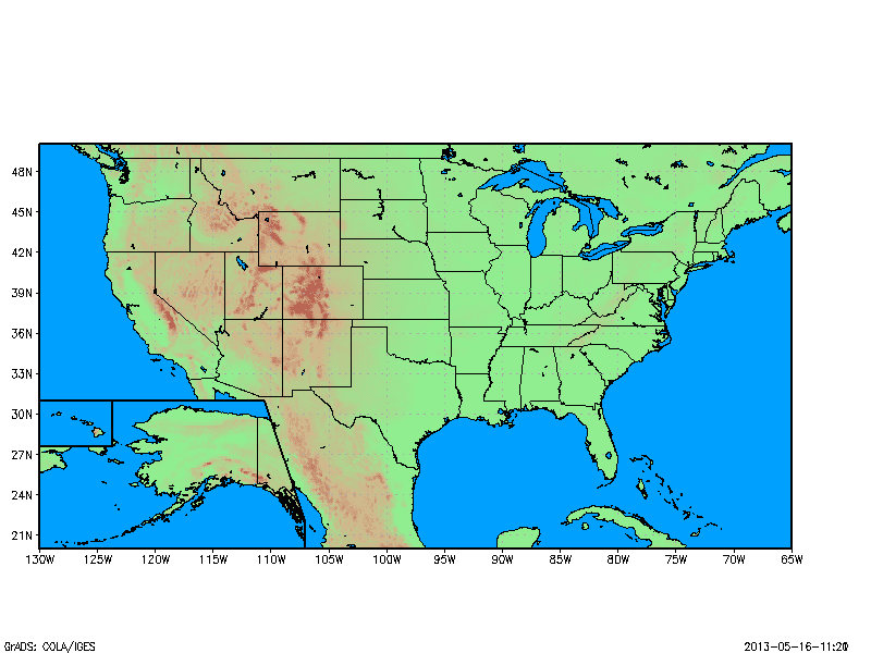
Script: us_map.gs; Draws and saves map of the United States with Alaska and Hawaii in the lower left corner

This script gives you the ability to generate the classic US map that has helped convince countless of Americans that Alaska is really an island near Mexico, and not a giant landmass far to the north.


Required Arguments: -var: chosen plot variable

Options:   -help(-h):  Pulls up Help Page
                  -base(-b): Uses Basemap options, you must follow this option with an "O" or "L"
                  -iname   : Sets name of output image, you must follow this with an image name
                  -xsiz      : Toggles the number of pixels in x
                  -ysiz      : Toggles the number of pixels in y
                  -bcol     : Toggles the color of the basemap'

Example Usage: 'us_map rose -b O -iname topomap.png'
                             -Plots the topography with masked out ocean and saves to the image: topomap.png

US Topomap made using us_map.gs

Note, when using us_map.gs, the lat/lon boundaries are set within the script, so you cannot set these before hand.  Also, be sure to set your other plot options before using us_map.gs (e.g., page area, contour levels, etc.).  Lastly, us_map.gs turns off the x and y labels to plot the boxes for Alaska and Hawaii, so you may need to turn them back on after using us_map.gs.  Also, please report any bugs so that this script may be fixed in future versions.

Download us_map.gs

Read More

Tutorial: How to make a basemap using GrADS

Note: This tutorial was updated October 2019 to reflect the fact that the Grads Data Server has been discontinued, so the online access of the terrain data through monsoondata.org is no longer available.

This tutorial was first published in 2013, with a tutorial on how to create a basemap of the United States.  In updating the tutorial for 2019, I have decided to alter the tutorial to focus on a different region of the globe, Europe to be specific.  Functionally, the concepts are the same (see images below).

Introduction:
Basemaps are a great way to add some color and vibrance to your weather maps.  GrADS allows you to output data onto a pre-generated .png image (i.e., a basemap) instead of redrawing the map everytime you want to make a figure.  This can be a big time saver if you're making several images in sequence.  This tutorial will show you how to make a basemap in GrADS using the 'basemap.gs' script and accompanying polygon files to mask the ocean..  You will learn how to:

1. Download and open netCDF topography data from NOAA 
2. Use the and the "basemap" script from the GMU GrADS Script Library to mask out oceans. 

It is recommend that you check out the basemap overlay tutorial if you are unfamiliar with GrADS basemaps.

Finished Basemap: 2013 Tutorial

Finished Basemap: 2019 Tutorial

So, for this tutorial you must download the following files from the GMU GrADS Script Library.

• basemap.gs
• lpoly_lowres.asc
• opoly_lowres.asc
• lpoly_mres.asc
• opoly_mres.asc
• lpoly_hires.asc
• opoly_hires.asc

In addition to these scripts, it is recommended that you have the color.gs and/or the colormaps script your personal script folder so you can use the same color settings as this tutorial.

Where to get the data:
While the GDS has been discontinued, you can still access high resolution (1min) topography datasets in netCDF format from NOAA.  Simply access this link and download either the full ETOPO1 (netcdf) file, or use the NCEI "Grid Extract Tool" to subset the data to a geographic region of your choice.  If you're using the Grid Extract Tool it will look similar to the screen shot below.

Screen shot of grid extract tool.

Once you have the netCDF (etopo1.nc) file locally, move it to your own data folder: (e.g., home/grads_data/terrain/).

How to make the basemap:
Basemaps are fairly easy to make, and can essentially be boiled down to three simple steps.

1. Load the topography data and set a domain.
2. Define a topography color scale (this is why we need color.gs)
3. Fill in the water areas using the ".asc" files

Step 1: Load the topography data and set a domain:

This is probably the most important step in making a basemap.  In order to use the basemap later for your weather maps, you must know a) The lat/lon boundaries, b) the size of the image in pixels, and c) the GrADS page area of the map (set using the 'parea' command).  I strongly recommend that you write down your lat/lon boundaries, your page area coordinates,and your x and y pixel size for saving the image so that you know how to match data on top of the map.

    'set display color white'
    'set mpdset hires'
    'clear'
    path = 'home/grads_data/terrain/' ; *or whatever your path to the etopo1.nc file is.
    'sdfopen 'path'etopo1.nc'

You can run a "qfile" on the data to look at the metadata if you would like, but it's not necessary for this tutorial.

Now to set the actual domain.  So, to make the image above, we will set the domain for the United States.  We will do this using the 'set lat' and 'set lon' commands.

  'set lat 30 60'
  'set lon -16 35'
At this point, we have our file open and our domain set.  So the last thing we need to do before moving on to step 2, is define our page area.  Remember this is important, so you know how to scale your weather maps in GrADS to fit on this image.  We do this using the 'set parea' command.  For the above image, the page area is set by:

   'set parea 0.5 10.0 0.5 7.5'

Now that we have our area, we can move on to step two.

Step 2: Define a Topography Color Scale

This is very easy with the color.gs script, all you need to do is pick out a range of colors.  For the old US map, we used the color.gs script to make a color scale that transitioned from light green to brown, that fit the range of topography in the US (0 to ~4000 meters).

    int=(4100-200)/50       ;*int sets the interval used for topography, this scale sets 50 intervals.
    'color 200 4100 'int' -kind lightgreen->tan->brown'

For the 2019 update, I chose to use the colormaps script to define the "terrain2" color scale as follows:

  'colormaps_v2 -map terrain2 -levels 0 3500 100'

Choosing a color scale is entirely, up to you, but the above options look nice to me.  Once the color scale is set, simply display the variable.


Now, our basemap is starting to take shape and we are set to move on to the final step.

Step 3: Fill in Water areas
This is the last step, and the only step that involves the use of basemap.gs.

To fill in the water areas, you will need to run the basemap.gs script as such:

    'basemap O 11 1 M'

In this command, the O stands for Ocean, so the script will fill in bodies of water.  The two numbers correspond to the fill and outline colors respectively.  11 for medium blue and 1 for black.  Lastly, the M stands for medium resolution, so this will use the file opoly_mres.asc to fill in the ocean.  The reason to use mres instead of hires, is because the hires oceans only cover the oceans around North America, so since this tutorial looks over at Europe, you need to use mres.

Now, that you have a nice looking basemap, all thats left is to save the image using the 'printim' command.  Be sure to specify the image dimensions, so that you can match them later when you save GrADS output over your basemap.

    'printim img_name.png x800 y600 png'

And that's it, that's all there is to it! You now have a nice, elegant basemap to serve as a background for your GrADS output.  To learn more how to output GrADS data onto your basemap, check out this tutorial.

Note: This example script is for the 2013 tutorial with the broken GDS link.

Download Example script

Read More

Tutorial: Overlay image on basemap image using GrADS

This tutorial teaches you how to save GrADS output onto an already existing image, a basemap.  This allows you to bring more color and vibrance to your weather map by adding, for example, topographic maps underneath of your weather data.  The use of basemaps can transform the image on the left to the image on the right.

Before Basemap

After Basemap

Before we get started with the tutorial, it is recommended that you learn how to make your own basemaps (see tutorial on making basemaps here).  However, if you want to skip learning how to make basemaps for now, I will provide the basemap needed for this tutorial.  The basemap provided will be the same basemap used in the above example.  To download this basemap to your computer, simply right click on the image below and choose "Save Image As..." and save it to your GrADS folder.

Save this image, as your basemap for this tutorial

So, now that you have your basemap, lets get started.  Plotting data onto a basemap is very simple, and requires very little extra code.  All you need to do is add a few extra options onto the 'printim' command, when you are outputting your data to an image.

• Normal: 'printim img.png png x800 y600'
• Basemap: 'printim img.png png x800 y600 -b basemap.png -t 0'

The options -b and -t, respectively, stand for 'basemap' and 'transparency'.  After the -b you must indicate the path to the basemap image, and after the -t you must specify which color to make transparent.  You can find out this number by querying the shading information through the 'q shades' command, or simply specifying this number through the 'set ccols' and 'set clevs' command.

And that's pretty much all there is to overlaying your data onto a basemap.

There are however a few things to watch out for.  Since all you are essentially doing when you include the -b option, is printing your GrADS plot onto a preexisting image, you need to make sure all the image dimensions match.  To do this there are really only three things that you need to remember:

1. Your GrADS page area (parea) matches the page area on your basemap
2. Your image dimensions are equal (you can get your image dimensions by right clicking your image and looking at 'properties')
3. Your lat/lon boundaries must be the same between the basemap domain and the GrADS domain

If these three conditions are not satisfied, you will end up with an overlay that does not coincide with your basemap (see below image for an example of what this looks like)

Incorrect!

Now, that you have an idea on how to do it, here are the correct dimensions for the basemap provided here.

Image Dimensions: x=800px, y=600px
Parea: '0.5 10.0 0.5 7.5'
latitude: 22, 51
longitude: -128, -65

So if you were to use these dimensions in a script to plot radar, your code might look like:

     'set mpdset hires'
     'set lat 22 51'
     'set lon -128 -65'                                                        ;*Depending on the dataset, you may need to add 360 to this
     'set display color white'
     'clear'

     'set parea 0.5 10.0 0.5 7.5'                                                  ;*Note the page area is equal to the basemap
     'set gxout shaded'
     'set ccols 0 14 4 11 5 13 19 7 12 8 2 6'                                ;*Note that the 0 is the specified transparent color
     'set clevs  5 10 15 20 25 30 35 40 45 50 55 60 65'
     'd radar'
     'printim img.png png -b basemap.png -t 0 x800 y600'       ;*x800, y800 correspond to the image dimensions


That about does it for this tutorial, you should now be able to overlay images onto preexisting basemaps.  And just for fun, and so you know, your background image does not necessarily have to be a map.

I hope you enjoyed, and found this tutorial useful!

 Download example script

Read More