Tutorial: The difference between self describing and non-self describing NETCDF files, and how to write them

In writing posts for this blog, I try my best to avoid what could be considered "mission creep," or writing coding tutorials that at best only tangentially related to GrADS.  This tutorial is verging upon what could be considered mission creep and has as much to do with teaching "good data" practices as it does with teaching GrADS skills.  Furthermore, there are no GrADS scripting lessons to be learned here, and the only code I provide is written for Python. 

All that said, in this tutorial, I will be showing you how to write NETCDF files that can be read using GrADS using both the self describing 'sdfopen' and non-self describing 'xdfopen' commands. I do this because, you may one day find yourself with some gridded data set that you want to plot using GrADS, however this data set may be in a text file format, or perhaps maybe you need to perform higher level calculations on the data that cannot be performed in GrADS before you display it.  While you could write the data out as a binary data file with a GrADS control file, maybe you are more comfortable with the NETCDF format (I know I certainly am).  Plus there are other benefits to using NETCDF instead of binary; one example is cross compatibility. NETCDF files can be read in with pretty much any data analysis software, so not only can you read your file in GrADS, but you can read it in with Matlab, IDL, R, Python, etc., as well.

What makes a NETCDF file self describing?

It's all about the metadata!  Metadata is often referred to "data about the data."  For example, metadata includes things like:

• The data and time a file was created
• What data is in the file
• Units of variables within the file
• Information about the coordinates (e.g., lat, lon vs. x,y)
• If the data file is for model output it might include information such as 

• Resolution, parameterizations, time step

Metadata is super important, and learning how to include it in any data set you are producing/sharing is a critical skill in a scientific career.  We are lucky in meteorology because there have been solid efforts to standardize metadata practices in the past couple of decades.  Now, NETCDF makes it very easy to provide good metadata, so there is no excuse not to do it.  So if nothing else, I hope to get that point across to you with this tutorial.  To really drive this point home, here is a meme.

 

To make a file self-describing (that is such that GrADS can read the file in with NO accompanying control file required using the 'sfdopen' command) the metadata including in the NETCDF file must adhere to the COARDS data standards: More information on COARDS here.  Personally, I didn't find this website all that useful when figuring out how to make self-describing NETCDF files, but it does provide some nice background.

How to write a self describing NETCDF file (SDFOPEN)

Here I will provide the key metadata required to write a self-describing NETCDF file.  The example, I provide is sub-setting the first 24 hours of GFS temperature data from the 00z December 30th 2015 run.  If you choose to try and reproduce these results, you will need to update the date.  I will us python to read in the data from the GrADS Data Server (GDS) and to write the local NETCDF file.  You could use any program of your choice to do this, so long as it reads and writes NETCDF files.  The python script is included in this tutorial.

So the most important thing to understand when writing your datafile is that your coordinate dimensions and accompanying dimension variables (e.g., lat,lon) adhere to the COARDS guidelines, otherwise GrADS will not open your file.  For example, you might get an error like:

     gadsdf: SDF file has no discernable Y coordinate

The metadata for the non-dimension variables (e.g., temperature, u,v) is more up to the person writing the file.

Assuming you know how to read in the NETCDF file and data from the GDS, in python:

   datafile='http://nomads.ncep.noaa.gov:9090/dods/gfs_0p25/gfs20151230/gfs_0p25_00z'
   cdata=netCDF4.Dataset(datafile,'r')
 
To start writing the file, we will first look at the dimensions and dimension variables.
You must include the following dimensions and variables in your NETCDF file:

• lat
• lon
• time
• lev

 In python you will make these dimensions and variables as such:

   newdata=netCDF4.Dataset(newfile,'w')
   newdata.createDimension('lat', len(lat[lmin:lmax]))
   newdata.createDimension('lon', len(lon[lomin:lomax]))
   newdata.createDimension('lev', len(lev[:]))
   newdata.createDimension('time', 8)

Where lmin,lmax,lomin,lomax are indices that mark your subset boundaries.
Then in addition to creating the dimensions, you must make the variables as well (For example latitude):

   latvar=newdata.createVariable('lat','f8',('lat'))

Now you need to populate latvar with metadata.  To determine what metadata you need, I simply printed out the 'lat' variable from within the GDS datafile as this datafile is self-describing and adheres to the COARDS standards.  If you've seen my other tutorials I often access these files using the 'sdfopen' command.  In doing that, I get the following (again this will look different if you aren't using python):

<type 'netCDF4.Variable'>
float64 lat(lat)
    grads_dim: y
    grads_mapping: linear
    grads_size: 721
    units: degrees_north
    long_name: latitude
    minimum: -90.0
    maximum: 90.0
    resolution: 0.25
unlimited dimensions:
current shape = (721,)

These are the metadata that you need to include for the latitude variable in your NETCDF file.  The dimensions will change, because you are sub setting the data, but things like 'grads_dim' and 'grads_mapping' need to be the same.  In python adding metadata to a NETCDF variable is easy:

   latvar.grads_dim='y'
   latvar.grads_mapping='linear'
   latvar.grads_size=str(len(lat[lmin:lmax]))
   latvar.units='degrees_north'
   latvar.long_name='latitude'
   latvar.minimum=str(lat[lmin])
   latvar.maximum=str(lat[lmax])
   latvar.resolution='0.25'
   latvar[:]=lat[lmin:lmax]

Again, remember with the sub setting, the lmin and lmax indices are required to match the output file.
Now if I print out MY latitude variable within the output NETCDF file it looks similar to the GDS file with only minor differences:

<type 'netCDF4.Variable'>
float64 lat(lat)
    grads_dim: y
    grads_mapping: linear
    grads_size: 200
    units: degrees_north
    long_name: latitude
    minimum: 10.0
    maximum: 60.0
    resolution: 0.25
unlimited dimensions:
current shape = (200,)

You will need to do the same thing for the other dimension variables (lon,lev,time) with a few minor differences.  I don't explicitly show the steps here to save space and redundancy.  You can find the steps written down in the accompanying .py file.

Once you have your dimension variables, you need to add the temperature variables.  In the example, I have you add both the 2 meter temperature and the temperature as a function of pressure level.  This is to show you how to add variables with differing dimensions.

As I stated earlier, there are fewer restrictions for these variables than the dimension ones.  But it is still a good practice to add metadata.  When printing out the GDS 'tmp2m' var, you get this:

<type 'netCDF4.Variable'>
float32 tmp2m(time, lat, lon)
    _FillValue: 9.999e+20
    missing_value: 9.999e+20
    long_name: ** 2 m above ground temperature [k]
unlimited dimensions:
current shape = (81, 721, 1440)

So for our variable, we will try to match this as close as possible:
  gtmpvar=newdata.createVariable('GTMP','f4',('time','lat','lon'),fill_value=9.999E20)
  gtmpvar.long_name='2 Meter Temperature'
  gtmpvar.units='K'
  gtmpvar[:]=var1[:8,lmin:lmax,lomin:lomax] ## Add the actual data from the GDS file

And that's it for the 2 meter temperature.  Now, you can do the exact same thing for the vertically varying temperature with only minor changes:
   tmpvar=newdata.createVariable('TEMP','f4',('time','lev','lat','lon'),fill_value=9.999E20)
   tmpvar.long_name='Pressure Interpolated Temperature'
   tmpvar.units='K'
   tmpvar[:]=var2[:8,:,lmin:lmax,lomin:lomax]

The big difference here, is that in the dimensions section of the createVariable function includes a dimension for 'lev'.

When you are done, close out your file and you can then open it in GrADS using the 'sdfopen' command.  Then if you display the temperature data, you should get something that looks like this:

How to read and write a NON self describing NETCDF file (xdfopen)

If you want to read a file that is not self-describing into GrADS, you need to include a control file.
Essentially, you need to treat the NETCDF file as if it were a binary data file.

Now for this tutorial, we will run through the exact same process, highlighting the differences in how we write metadata to the NETCDF file.

Starting with the dimension variables, we will no longer include the metadata that we did for the self describing file:

    newdata=netCDF4.Dataset(xdffile,'w')
    newdata.createDimension('lat', len(lat[lmin:lmax]))
    latvar=newdata.createVariable('lat','f8',('lat'))
    latvar[:]=lat[lmin:lmax]

Similarly, I'll skip the rest of the dimension variables, but as you see, all I did was define the variable and add the data to it.  For simplicity, and since it doesn't matter, I'll keep the temperature variables as they were in the self describing example.

Now the NETCDF file is created.  If however you try to open this file using the 'sdfopen' command, you will get an error.  So we need to create a control file.

The control file can be easily written using python (as in this example) or whatever program you are using.  I'm going to copy the code to write the control file below, and explain it after.

    ### Now write the control file ###
    xdfctl='C:/OpenGrADS/xdffile.ctl'
    xdflocal='xdffile.nc'
    xdf = open(xdfctl, 'w')
    xdf.write('DSET ^' + xdflocal +'\n')
    xdf.write('TITLE XDF example File 00z30dec2015 \n')
    xdf.write('UNDEF 99999.0\n')
    xdf.write('XDEF lon '+str(len(lon[lomin:lomax]))+' LINEAR ' + str(lon[lomin]) +' 0.25\n')
    xdf.write('YDEF lat '+str(len(lat[lmin:lmax]))+' LINEAR ' + str(lat[lmin]) +' 0.25\n')
    xdf.write('ZDEF lev '+str(len(lev[:]))+' LEVELS ')
    for i in lev[:]:
        xdf.write(str(int(i))+' ')
    xdf.write('\n')
    xdf.write('TDEF time 8 LINEAR 00z30dec2015 3hr\n')
    xdf.write('VARS 2\n')
    xdf.write('GTMP=>GTMP 0 99 2-meter Temperature [k]\n')
    xdf.write('TEMP=>GTMP '+str(len(lev[:]))+' 99 Temperature [K]\n')
    xdf.write('ENDVARS')
    xdf.close()

The most important take away to learn about writing a control for a NETCDF file is that you match the variable/dimension names in the control file to the variable/dimension names in the NETCDF file (case sensitive).

For example: 'GTMP=>GTMP' will only work if there is a variable in the NETCDF file called 'GTMP'.  Similarly, following the XDEF definition, you need to point to the longitude variable (lon) in the NETCDF file.  This is different than writing out control files for binary datasets which don't require anything after XDEF.

Other than that, you see some other things, the levels are defined in a special way since the vertical coordinate is not incremented linearly.  Also the lat/lon sizes are not hard coded, to allow you to make bigger or smaller spatial subsets without a lot of extra work.

Open the control file in GrADS using the 'xdfopen' command:

'xdfopen xdffile.ctl'

A few notes on using the control file:

Note that the coordinate data is not actually read
from the NETCDF file, it is inferred from the control file.  So it is important that the resolution and the starting points are right, otherwise you will get an incorrect result, even if your longitude data is correct in the NETCDF file.  For example, comparing the correct (0.25) resolution to an incorrect resolution (0.45) gives the two different maps shown on the right.  So get the resolution right!

One final note: This kind of control file only seems to work with nice rectangular datasets.  That is lat/lon coordinates that vary independently from one another.  If your lat/lon grid does not vary independently (i.e., longitude is a function of y and visa-versa), then using this method will warp tour map projection.  In these situations it is recommended that you write your data out to a binary file with the PDEF option.  I have yet to get the PDEF option to work with a NETCDF file.






So that is it for the tutorial, hopefully you have a better understanding regarding the difference between self describing and non self describing NETCDF files, and how to write and open them in GrADS.  No GrADS scripts to download here, but a full python script (version 2.7) is included that will reproduce the files and plots generated in this tutorial.  You will need the netCDF4 module installed for this script to work however.  Numpy and sys are standard I believe.  Also you may need to update the date.

Download Python Script here

Read More

Tutorial: Shapefile; A look at the DBF file.

This is the 2nd tutorial on using shapefiles in GrADS.  If this is your first time using shapefiles in GrADS, it is recommended you check out this tutorial.  This tutorial will dig a little deeper and look at the 'q dbf' command to look at the different shapefile properties.  For this tutorial, we will take a break from the usual focus on weather data, and instead focus on politics!  What we will do is draw the United States colored by which way each state voted in the 2013 presidential election.

Blue: Democrat, Red: Republican

So, to start you first need to download the required shapefile: Shapefile
Once you have this file put in your shapefile folder, we can begin.  Now we do need to open a file to get the environmental scaling, but that's all we need it for.  I'm going to use a simple GFS file from the GrADS Data Server.

    'sdfopen http://nomads.ncep.noaa.gov:9090/dods/gfs_hd/gfs_hd20130512/gfs_hd_00z'
    'set lat 22 50'
    'set lon -125 -68'
    'set clevs 10000000'
    'd pressfc/100'

Now, we have our file open and our map set up.  Now we are ready to plot our shapefiles.  However, we need to specify the color of each state.  This is where the 'q dfb' command.  The 'q dbf' takes a look a the database (.dbf) file that came in the shapefile zip folder, which is essentially the metadata.  So for this example, we would query the database file of the state shapefile.

    'q dbf Shapefiles/s_06se12.dbf'
   say result

What you will see is a list of information separated by commas.  What this information tells you, is the state abbreviation, shapefile id number, lat/lon, state name.  So, all we need to do, is extract this information and compare it to our previous knowledge of who won the election.  The hardest part of this is dealing with the fact that each value is separated by a comma instead of a space; we can't just use the 'subwrd()' command.  So, since we know that arrays can be set with strings as well as numbers, we can simply set a list of different colors, corresponding to each state abbreviation.

The first few numbers might look like:
    *2=Republican
    *4=Democrat

    col.AL=2
    col.AR=2
    col.AZ=2
    col.CA=4
    ....
    ....


Once, you have your list set, we simply need to loop through each shape within the shapefile, and determine its state abbreviation, then set the shapefile fill color to the color corresponding to the list above.

    i=2
    check=1
    while(check=1)
      'q dbf Shapefiles/s_06se12.dbf'
      line=sublin(result,i)
      if(line='' | line='(NULL)');check=0;else;

        com_count=1
        vars=1
        while(vars<=3)
          com_check=1
          len=1
          c=com_count
          while(com_check=1)
            comma=substr(line,c,1)
            if(comma=',');var.vars=substr(line,com_count,len-1);com_check=0;endif
            if(comma='' & vars=11);var.vars=substr(line,com_count,len-1);com_check=0;endif
            len=len+1
            c=c+1
         endwhile
         com_count=com_count+len-1
         vars=vars+1
       endwhile
       state=subwrd(var.3,1)
       'set shpopts 'col.state
       'draw shp Shapefiles/s_06se12.shp 'i-2
      endif
     i=i+1
   endwhile

This block of code may look complicated, but mostly it is just looking for commas within the string, and setting variables to the values in-between each comma.  You will also see the option "i-2" added on at the end of the 'drawshp' command.  This is telling GrADS to only plot the shapefile that has the id number i-2.  Since I starts at 2 (the first line of data in the shapefile), and since the first ID number is 0, we need to offset the pointer by 2.  So what this loop does, is loop through all of the shapes in the shapefile, and set the color to the list prescribed at the beginning of the script. 

If you run this script in GrADS, you will see a the shapes start to show up colored on the map.  So, that does it for this tutorial, hopefully it helped you work a little bit with the 'q dbf' command. 

Download Example Script Here

Read More

Tutorial: Draw arbitrary cross-section with terrain in pressure coordinates using GrADS

As mentioned in the introductory post, one of the major deficiencies with GrADS, is that drawing arbitrary vertical cross-sections is not an easy task.  There are however work-arounds to do this, but they can be quite complex, especially when including terrain.  This tutorial will guide you step by step through the process of plotting an arbitrary cross section in GrADS with terrain in pressure coordinates.

Essentially, to plot arbitrary vertical cross sections in GrADS, you have to collect your (z-varying) data at each lat/lon point in your cross section, and then re-grid that data before plotting it.  The g2stn(), and the coll2gr() functions in GrADS help you along with doing this.  For this tutorial, I am going to start by borrowing the code from this link and change around a couple of variables.  In this section will provide a basic walk through of what this code is doing.  Once we have gone though this code, I will show you my work around to plotting terrain, which is similar to some of the other work-arounds out there, but I think mine works a little faster.


     'sdfopen http://nomads.ncep.noaa.gov:9090/dods/gfs_hd/gfs_hd20130512/gfs_hd_00z'
     'set x 1'
     'set y 1'
     'set xlog on'
     'set lev 1000 100'
     lon1 = -95.0
     lon2 = -90.0
     lat1 = 55.0
     lat2 = 15.0
     lon = lon1
     'collect 1 free'
     while (lon <= lon2)
       lat = lat1 + (lat2-lat1)*(lon-lon1) / (lon2-lon1)
       'collect 1 gr2stn(rhprs,'lon','lat')'
       lon = lon + 1
     endwhile

     'set lon 'lon1' 'lon2   
     'set clab on'
     'set gxout shaded'
     'color 50 100 2 -kind black->lightgreen->darkgreen->darkblue'

*If you don't have color.gs:
*         'set clevs 40 50 60 70 80 90 100'
*         'set ccols 0 3 4 5 6 7 9 10'
*--------------------------

     'd coll2gr(1,-u)'


So, this code is pretty similar to the example shown in the link provided above, but with a few minor differences, for example we are plotting relative humidity, instead of pv.  Also, I used the world dimension to set the x-axis for the arbitrary cross-section.  This is fairly meaningless, as it will still just plot the values that you have there, regardless of the dimensions.  Lastly, I used color.gs to do the RH color scale.

Lets break down this code a little bit, so that you have an idea as to what you are doing with it.  The first thing you see below the plot scaling is the declaration of your longitude and latitude boundaries.  To make arbitrary cross sections, you must declare your boundaries.  Once the boundaries are declared, you see the 'collect 1 free' command.  This basically, tells GrADS that you are emptying out the grid-collection numbered "1".  So, if there is anything in there, you are freeing this variable.  If you wanted to plot more than one variable, you would put another 'collect' command for a different number, e.g., 'collect 2 free'.  Assuming, you are only plotting relative humidity, the loop will run through (slowly if I may add) collecting the z-varying variable at each lat/lon point.  You can see the latitude is really just a linear interpolation between your latitude boundaries.  Once you have collected all of your data, the dimensions are set on the x-axis (longitude), and the variable is plotted at all vertical levels using the coll2gr() function.  And that is about as simple as this gets, you can see the resulting image below.

Arbitrary cross-section varying in both lat/lon.

As you can see, it's not too much to look at, I did the plot over a small area so to reduce computational time, but this is basically what you get if you use the method described in the above link.

Now, how about adding terrain.  This is tricky business because terrain (or surface pressure in pressure coordinates) is not a z-varying variable.  So, unfortunately, it is not as simple as adding terrain into another collection variable.  Once again, similar to plotting terrain on a log scale, we need to pull some tricks!  Basically, what we are are going to do, is scale the environment, and use the 'q w2xy' command and generate a bunch of vertices to use in a polygon fill.  Then to draw the terrain, we simply draw our polygon.

So, here is the code for drawing a cross section with arbitrary terrain.

    'sdfopen http://nomads.ncep.noaa.gov:9090/dods/gfs_hd/gfs_hd20130512/gfs_hd_00z'

    'clear'
    'set grads off'
    'set zlog on'
    lon1 = -115.0
    lon2 = -95.0
    lat1 = 40.0
    lat2 = 35.0
    lon = lon1

    terrain_arr=''

    'set lat 'lat1
    'set lon 'lon1' 'lon2
    'set lev 1000 100'
    'set gxout shaded'
    'd rhprs'
    'draw title Temporary Scaling Environment'

    'collect 1 free'
    'collect 2 free'
    'set x 1'
    'set y 1'

    say 'collecting station data'

    'q gxinfo'
    xline=sublin(result,3)
    yline=sublin(result,4)
    xs=subwrd(xline,4)' 'subwrd(xline,6)
    ys=subwrd(yline,4)' 'subwrd(yline,6)


    while (lon <= lon2)
       'set lev 1000 100'
       lat = lat1 + (lat2-lat1)*(lon-lon1) / (lon2-lon1)  
       'collect 1 gr2stn(rhprs,'lon','lat')'

       'set gxout print'
       'set lat 'lat
       'set lon 'lon
       'set lev 1000'
       'd pressfc/100'
       press=sublin(result,2);press=subwrd(press,1)
       'q w2xy 'lon' 'press
       x=subwrd(result,3)
       y=subwrd(result,6)

       if(x<=subwrd(xs,1));x=subwrd(xs,1);endif
       if(x>=subwrd(xs,2));x=subwrd(xs,2);endif
       if(y<=subwrd(ys,1));y=subwrd(ys,1);endif
       if(y>=subwrd(ys,2));y=subwrd(ys,2);endif
       terrain_arr=terrain_arr''x' 'y' '

       lon = lon + 1
     endwhile

    say 'plotting data'
    'clear'
    'set lev 1000 100'
    'set lon 'lon1' 'lon2
    'set clab on'
    'set gxout shaded'
    'color 50 100 2 -kind black->lightgreen->darkgreen->darkblue'
    'd coll2gr(1,-u)'

    say 'drawing terrain'

     x1=subwrd(terrain_arr,1)
     y1=subwrd(terrain_arr,2)
    terrain_arr=terrain_arr''subwrd(xs,2)' 'subwrd(ys,1)' 'subwrd(xs,1)' 'subwrd(ys,1)' 'x1' 'y1

    'set line 15 1 1'
    'draw polyf 'terrain_arr


You can see the similarities to the code above, the variable is still collected and regridded using the g2stn() and the coll2gr() functions.  But now there is a lot more code relating to the drawing of the terrain.  Lets break this down.  The first extra command, is the one at the top that sets the variable terrain_arr=''.  This is going to be our polygon array.  We are going to populate this with a bunch of vertices corresponding to the terrain.  But first, we need to clear it.  Once we have cleared that array, we plot a "Dummy" cross-section to scale our environment.  Remember, it doesn't matter what our latitude is, because in the loop, we set the latitude for each variable, and our world coordinates vary in longitude and height.  But we can plot our dummy variable as such.  I also gave it a title, so to specify that it is just a temporary dummy plot.

      'set lat 'lat1
      'set lon 'lon1' 'lon2
      'set lev 1000 100'
      'set gxout shaded'
      'd rhprs'
      'draw title Temporary Scaling Environment'


Now, once we have our environment scaled, we move into our loop.  Here, we set our variables the same way, but then we need to get our terrain value converted from a world coordinate to a page coordinate.  We do that by setting the gxout to be print, and then setting the specific lat/lon coordinate.  Then we simply print out the surface pressure at this point, and use the 'q w2xy' command to convert that into page coordinates.  We then check to make sure the page coordinates for each vertex in our polygon falls within the plot area.  Then we simply build the array from there.

       'set gxout print'
       'set lat 'lat
       'set lon 'lon
       'set lev 1000'
       'd pressfc/100'
       press=sublin(result,2);press=subwrd(press,1)
       'q w2xy 'lon' 'press
       x=subwrd(result,3)
       y=subwrd(result,6)

       if(x<=subwrd(xs,1));x=subwrd(xs,1);endif
       if(x>=subwrd(xs,2));x=subwrd(xs,2);endif
       if(y<=subwrd(ys,1));y=subwrd(ys,1);endif
       if(y>=subwrd(ys,2));y=subwrd(ys,2);endif
       terrain_arr=terrain_arr''x' 'y' '

At the end of the loop, you should have a big long array filled, with x/y coordinates.  But we are not quite done.  We will need to close out our polygon.  So the last thing we do before drawing our polygon is add a couple more vertex values to it, so it runs back down and closes it off.  Then we simply draw the polygon. 


     x1=subwrd(terrain_arr,1)
     y1=subwrd(terrain_arr,2)
    terrain_arr=terrain_arr''subwrd(xs,2)' 'subwrd(ys,1)' 'subwrd(xs,1)' 'subwrd(ys,1)' 'x1' 'y1
    'set line 15 1 1'
    'draw polyf 'terrain_arr

And, voila! Your terrain is drawn on the map.  What's even more fantastic about this, is that you do not even have to pull any special strings to plot this in log coordinates.  This method works both ways.

To prove this works as intended, I am showing you two images below, both are the same E/W cross section with terrain, however one was made using the arbitrary cross-section method, the other, the simple GrADS command.  Also, for simplicity, I plotted it on a non-log scale, so to make the simple GrADS command easier.

Normal Method

Arbitrary Method

So, as you can gather, these plots are identical, and that is good, because if they weren't than the arbitrary method would not be correctly plotting the terrain.

A few final notes before wrapping up: 

•  The main issue with the plotting arbitrary cross-sections, is that it is slow if you are accessing the data online through, for example, the GrADS data server.  The plot above took ~5-10 minutes, this time will increase the more variables that you add to your plot.

• You need to be aware that the lon=lon+1 command can lower the resolution of your plot if your x grid-spacing is less than 1 degree of longitude.  For example, the above plot was made using the 0.5 degree GFS data so to ensure that my plots matchedin up, my longitude was increased by increments of 0.5: lon=lon+0.5.  You could add a simple 'q file' command to your script to get the grid-spacing and always set your longitude to increment that way, but bear in mind this can really increase your computational time, as you are collecting more points.

• There is more than one way to skin a cat: I want to note there are other methods to plot terrain on your arbitrary cross-sections, but I have found them to be slower than this one, as they require you loop through your data points more than once.  This method just requires one loop.  But other methods are perfectly acceptable as well, and will probably give you similar or the same results.
   

So that's it, this was a fairly long tutorial, but hopefully you have a better understanding how  to plot arbitrary cross-sections in GrADS.  Especially when it comes to including terrain in pressure coordinates.  I imagine you could probably carry this method over to height coordinates easily enough though.

Download Example Script

 

Read More

Script: Dynamic: Calculates temperature and vorticity advection, Q-vectors, deformation, geostrophic and ageostrophic winds, and Fronogenesis in GrADS

Usually, more advanced dynamic variables like frontogenesis and deformation are not included in the list of variables in your model output files.  Instead, it is up to the user to calculate them from the available wind and temperature fields.  Calculating these variables is complex and often requires a lot of steps using the various centered difference functions in GrADS.

Dynamic.gs calculates the following variables from the geopotential height, temperature, and horizontal wind.

Variable                           Name             Units                
-Geostrophic Wind     :    ug,vg             [m/s]   
-Ageostrophic Wind   :    ua,va             [m/s] 
-Q-Vectors                :    Q1,Q1           [pa/m2/s]   
-Temp Advection       :    tadv               [K/s]        
-Vort Advection         :    vadv              [-]         
-Frontogenesis         :    F                   [K/m/s]x10^9
-Fn Vector                :    fnx,fny         [K/m/s]x10^9
-Deformation             :    def1,def2     [m]         

The variables are then saved into the name, and you can plot them as normal variables.  However, since there are a lot of calculations to make in this script, the variables are only calculated for the current dimensions.  To calculate these values at all x,y,z,t points, simply set your dimensions to span the entire 4D domain.

Options:   -help: pulls up help page
                  -var : allows the user to point to specified height, temperature, wind variables
                            Default variables are: hgtprs, tmpprs, ugrdprs, vgrdprs


Example Usage: dynamic -var hgtprs tmpprs ugrdprs vgrdprs

This example will use the hgtprs, tmpprs, ugrdprs, vgrdprs variables to calculate the dynamic variables.

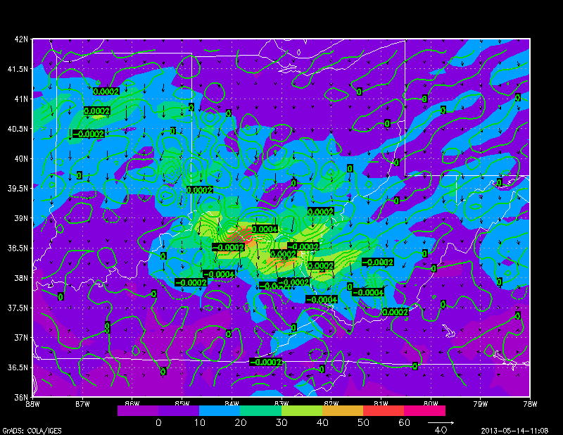
Example Image: NARR Shaded: Fronogenesis, Contoured in Green: Fn vector divergence, Vectors: Fn Vectors for 06UTC Feb 15, 2003

850-700mb average: Frontogensis, Fn Vectors, Fn Divergence, plotted for 06UTC Feb 15 2003

I chose this example to compare to the example used in this presentation.  Things seem to match up reasonably well.  Though I do urge some caution here, I am not (nor have I ever been) a dynamics expert, and some of the calculations were taken from either old GrADS scripts, or approximations of textbook equations.  Also, it is possible that the listed units are not 100% correct.  These caveats aside, I have been using this script to successfully diagnose areas of frontogenesis, and ageostrophic circulations from model output for quite some time, so I think overall it serves it's purpose well.  I post it now, with a newly added help page, and slightly cleaner code.

Download Dynamic.gs Here

Download Frontogenesis Example Here

Read More

Tips on using the finite differencing functions in GrADS (e.g., hdivg, and hcurl): Getting rid the undefined strip along the map boundary

The finite differencing functions in GrADS are pretty handy, especially when it comes to plotting variables such as divergence. The finite differencing function used in GrADS is called cdiff(), and what cdiff() does, is simply take the finite difference of a certain variable. For example, if you wanted to take the chance in u-wind in the x-direction, cdiff would be called as such:

    cdiff(u,x)

It is important to note, that this is not du/dx, as it is taking the chance in u from one grid point to the next, and not the physical distance.  If you wanted du/dx, you would have to multiply the denominator by the grid-spacing.  A good example of using the cdiff function can be found here.

GrADS includes a couple of commonly needed functions that use cdiff: hdivg(), and hcurl().  These function use the finite difference method to plot horizontal divergence and vertical vorticity respectively.  A common issue that people may come across while using this function is the appearance of a "blank strip" along the boarder where the data is not plotted.  An example of this strip is below.

GFS 700hPa divergence (hr-1)

It may be hard to notice here, but you can clearly see a strip of white along the boundary.  The reason this appears is simple enough, basically you are plotting a difference, and at the edge, there is only one point, so there is nothing to plot on the edge points.  The way around this is very simple.  All you need to do, is set the domain one grid point larger than you intend to plot, define your variable, then fix the domain to your plot size, and plot it.  That way, you define the finite difference at the edge of your domain before plotting.  Of course, this method relies on having the data outside of your desired domain.  Anyway, the code to do this is simple enough:

    'sdfopen http://nomads.ncep.noaa.gov:9090/dods/gfs_hd/gfs_hd20130512/gfs_hd_12z'

    'set lat 20 52'
    'set lon -127 -66'
    'set gxout shaded'
    'set mpdset hires'
    'set display color white'
    'clear'

    'set gxout shaded'
    'set lev 700'
    'define var = hdivg(ugrdprs,vgrdprs)*3600'

    'set lat 21 51'
    'set lon -126 -67'

    'd var'
    'cbar'

As you can see the lat/lon boundaries extend out just a little bit farther when defining the variable, then are shrunk when making the actual plot.  The resulting image is:

GFS 700hPA divergence (hr-1)

This image is very similar to the image above, but you now clearly see that there is no "blank" strip along the borders of the image.

The finite difference functions in GrADS can be useful for a whole number of different purposes.  Hopefully these quick tips will help you better use these functions in the future.

Read More

Tutorial: Use the tcorr function to create a map of regression/correlation coefficients in GrADS

Making a correlation map in GrADS is actually quite simple.  A regression/correlation map, is basically a map of regression and correlation coefficients plotted against a time-series of some variable.  The classic example is the monthly average time-series of El-Nino vs. surface temperature on the globe.  The example used in this tutorial will be 500mb height correlated with the 500mb height over the northeast U.S.  For this tutorial we will use the NCEP reanalysis data.

GrADS makes correlation maps very simple.  All you need is a data set that varies in both space and time.  The first step is to define your time-series variable.  In the interest of time and simplicity, I will just take the 500mb height at one point rather than average over a small spatial area, as is often done when doing these maps.  So lets open the data file and set our time-series variable!

    'sdfopen http://monsoondata.org:9090/dods/rean3d'
    'set t 1 636'
    'set lev 500'
    'set lat 44'
    'set lon 282'
    'ts_var=z'

The variable "ts_var" is our time-series variable, and basically we saved the time-series of geopotential height at 500mb at the lat/lon point of 44/282.  Now, we are going to use two intrinsic GrADS functions to plot the regression coefficients (shaded) and the correlation coefficients (contoured above 0.5).

So, to plot our coefficients, we use the 'tregr()' and the 'tcorr()' functions.  Both of these functions do essentially the same thing; you feed them a time-series variable, and a spatial variable, as well as time-constraints, and the function plots your coefficients.

Example:  tregr(x, y, t=1, t=50)

This variable takes the regression coefficients of spatial variable y and time-series x through the first 50 time-steps.  In our example of 500mb height our code looks like:
  
    'set gxout shaded'
    'set t 1'
    'set lat 0 90'
    'set lon 180 360'
    'd tregr(ts_var,z,t=1,t=636)'

    'set gxout contour'
    'set cstyle 2'
    'set cthick 6'
    'set ccolor 1'
    'set clevs 0.5 0.6 0.7 0.8 0.9 1.0'
    'd tcorr(ts_var,z,t=1,t=636)'

Most of the above code is for display of the contour variable; style, thickness, levels, but you can see the tregr() and the tcorr() functions used correctly.  If you are following along at home, the resultant map is plotted.

Shaded:Regression Coefficients, Contoured: Correlation Coefficients

So, what you can gather from this map is that the 500mb geopotential height is generally well correlated above 20 degrees N (r>0.8).  Furthermore, you can pick out the Rossby wave pattern in the regression coefficients.  In anycase, this example show give you an idea of how to make regression/correlation maps in GrADS.

Download Example Script

Read More

A look at the different map projections in GrADS

There are a number of different possible map projections you can use in GrADS, and you may be familiar with some, or all of them, or perhaps you are only familiar with the standard default lat/lon projection used.  This entry will be less of a tutorial and more of just a detailed look at the different map projections you can use in GrADS.  However, before we get started, we do need a little tutorial section, just so you know the syntax for setting the map projection.  Setting the map project is extremely simple: Use the 'set mproj' command and provide it with a map projection from the list below:

1: latlon      Lat/lon projection with aspect ratio maintained (default)
2: scaled      Lat/lon aspect ratio is not maintained; plot fills entire plotting area
3: nps         North polar stereographic
4: sps         South polar stereographic
5: lambert     Lambert conformal conic projection
6: mollweide   Mollweide projection
7: orthogr     Orthographic projection
8: robinson    Robinson projection, requires set lon -180 180, set lat -90 90
9: off         No map is drawn; axis labels are not interpreted as lat/lon

Example:
    'set mproj nps'

That's all there is to it.  Once you have set your projection, you set the lat/lon boundaries as you normally would using the default settings, although certain map projections have intrinsic limits associated with them, which we will explore here.  So, in order to make the examples shown below, we will very simply plot vorticity from the GFS on a bunch of different map projections.  So starting out with the following code we will get this basic image, on the default cylindrical map projection,

    'sdfopen http://nomads.ncep.noaa.gov:9090/dods/gfs_hd/gfs_hd20130513/gfs_hd_00z'
    'set gxout shaded'
    'set lev 600'
    'set mpdset hires'
    'd abs(absvprs)'

Vorticity on a Defualt latlon map projection

So, now that we have that out of the way, lets look at the other map projections.

Scaled:

The scaled map projection does not differ much from the default cylindrical projection, except that it gets rid of the aspect ratio.  Basically, using this option will squish, or elongate the map to fit your specified page area.  The image below shows the transition.  To show the different more dramatically, I set the lat/lon coordinates to -40 to 40 instead of -90 to 90.

latlon vs. scaled map projections

Personally, I don't have much use for the "scaled" map projection, but it is always an option if you need to fit stuff together.

North/South Polar Stereographic NPS/SPS:

The NPS map projection can be useful if you are looking down at the north pole.  Pretend basically that you have the northern hemisphere, and you flatten it.  This would be the north polar stereographic projection.  For the southern hemisphere, simply take the same concept and apply it.  Now, while this map projection does not set latitude boundaries, my rule of thumb has been to set the minimum(maximum, depending on your hemisphere) latitude to be the equator.  I have trouble getting information if I look at southern hemisphere values using an nps projection.  The example below shows each full hemisphere using each projection.  Latitude set from 0 to 90 and -90 to 0.

NPS vs. SPS

Now, you don't need to have longitude set to cover the entire globe either, or the entire hemisphere.

Lambert:

The best way to think about the Lambert map projection is as if the Earth was projected onto a cone.  In fact, often time this projection is referred to as a "conic" projection as well.  Anyway, imagine the Earth is projected onto a cone with the north pole at it's point.  The Lambert projection is basically what the map would look like if the projection was unwrapped and then flattened.  The Lambert projection requires, that your latitude boundaries exist in the same hemisphere, otherwise the projection won't work.  The below example, shows the Lambert projection applied to the northern hemisphere for the longitude coordinates from -180 to 0 (western hemisphere)

Lambert Projection

Mollweide:

The Mollweide projection is often used to show global maps, but in GrADS there are no specific requirements for the latitude/longitude boundaries.  This projection can be neat, as it sort or combines a spherical look with a cylindrical look, with the meridians converging at the pole.  This gives a neat almost 3D appearance.

Mollweide projection

Orthographic Projection:

The orthographic projection is another neat projection that gives a 3D spherical appearance.  In GrADS there are strict requirements for the orthographic projection.  Your latitude boundaries must span -90 to 90.  Additionally, your longitude coordinates must span 180 degrees, no more, no less.  You have the option of choosing your longitude boundaries, so long as they cover 180 degrees of territory.  The result is an image similar to this one.

Orthographic projection

Robinson Projection:

The last map projection I am going to discuss is the "Robinson" Projection (The "off" projection is not really interesting, so I'm not going to talk about it) The Robinson projection is similar to the Mollweide projection, but with the poles kind of flattened out.  This is another commonly used map projection.  In GrADS this projection requires that lat/lon boundaries cover the entire globe.  Lat=-90 to 90, and Lon=-180 to 180 (0 to 360).

Robinson projection

So that's it for the different map projections in GrADS.  As always, each projection is useful depending on the situation, the map, the variable plotted, etc., etc.  I hope this post has given you a little more information regarding each different type of projection.  Just remember that some of them require specific lat/lon boundaries.  Aside from that, picking the right projection is just a matter of trial and error.

Read More

Tutorial: Two different methods for array syntax in GrADS

Arrays can be an extremely useful tool when using loops in GrADS.  Arrays reduce the number of lines in your code by a potentially large amount.  For example, if you wanted to plot soundings at a number of different locations: Without arrays, you would either need to have a separate segment of code for each location, or put a bunch of conditional statements in a loop to determine which location to set your coordinates to.  With arrays however, you can simply point to each new location using one single block of code, and no conditional statements.  If you are at all familiar with computer programming, in any language, you are almost certainly aware of the benefits of arrays.  This tutorial will be fairly short, and provide you with an idea of how to use the different array syntax methods in GrADS.

So basically, GrADS allows you to use arrays that are really only useful in loops, or potentially conditional statements.  The arrays in GrADS can't be used in liner algebraic operations, at least not easily.  I suppose you could put something together that might work, but then again what would be the point?  But in terms of telling the program to point to certain array values, the array syntax in GrADS is plenty sufficient.  There are two different methods to declaring and using arrays in GrADS that I work with.  I will explain each method, and give a little bit of information regarding their uses, including a couple of examples.

Method 1:

The first array syntax in GrADS uses the period (.) to indicate array values.  This is the simplest way to do arrays in GrADS, and I have found it sufficient nearly 100% of the time for what I want to do.  It is important to use the period syntax, instead of other possible separators (e.g., the underscore), as the period will separate the name and number in a loop.  The below example shows three different array expressions, one correct and two incorrect.

    array.1=5    ;*Correct
    array_1=5  ;*Incorrect
    array1=5    ;*Incorrect

    i=1

    say array.i
    say array_i
    say arrayi
The output from the following will be:

    5
    array_i
    arrayi

Basically, the period allows the variable "i" to be read as the number, the other two syntax expressions simply read the "i" as part of the variable name.

A few other notes about this GrADS array syntax: It is important to know that the array syntax here is very basic, and you aren't really declaring "arrays", what you're doing is simply declaring a bunch of variables, each with a period in the suffix, and then pointing to the names separately depending on the value of the suffix.  So sticking with the above example, these commands do not work:

   array=[5, 4, 3, 2, 1]  ;*No!

   say array.1
   say array.2

This does NOT output:

   5
   4

In fact, this script won't even run, you will just get an error  Also, this is no good:

  array.1=5
  array.2=4
  array.3=3

  say array

While this code will not give you an error if you try to run it, the output will NOT be:

  5 4 3

it will instead be:

  array

Get the idea?  Basically, you are just naming stuff, not really declaring arrays in the traditional sense.  That's pretty much it for this array syntax.  Now, this syntax can be exploited in a number of different ways, you can do 2D, or 3D or nD arrays, as long as each value is separated by a period.  Also, the values after the period do not necessarily have to be numbers.  The below examples will show you a few possible array expressions.

Basic Example: 

   x.1=5
   x.2=6
   x.3=15
 
   i=1
   while(i<=3)
      say x.i
      i=i+1
   endwhile

output:

   5
   6
   15

2D Array:

    x.1.1=15
    x.1.2=14
    x.2.1=12
    x.2.2=10

    i=1
    while(i<=2)
       j=1
       while(j<=2)
          say x.i.j
          j=j+1
       endwhile
       i=i+1
    endwhile

output:

   15
   14
   12
   10

 
Array Using Words:

x.array=15
word='array'

say x.word

output:

    15


That's it for the first method of arrays in GrADS, now onto the 2nd method!

Method 2:

This method is a little bit trickier to follow, but gives you a little better simulation of normal array syntax.  That being said, this part of the tutorial is actually much shorter than the above, as there aren't really as many variations of it.  This method, is basically to use the 'subwrd' command to point to values in a specified variable.  The 'subwrd' command basically scans a string and breaks it up into values separated by the space.  All you need to do is supply the function with the name of the string, and the word you are looking for.  For example, the code:

    array='5 10 15 20 25 30'
    say subwrd(array,4)
   say subwrd(array,1)+subwrd(array,2)

Would output the 4th word from this variable:

    20
    15

One of the benefits of using this syntax is that you can print out the array as a whole using the say command.  Another benefit is that you can really reduce the number of lines in your script this way vs. the 1st method.  Also, since GrADS is pretty good about automatically converting strings to floats, you can declare a string of numbers, and still do mathematical operations with each number. One drawback is that you can't really do multidimensional arrays this way.  Also if you are using names, you can't include names with spaces in them, since the 'subwrd' command uses spaces as delimiters between each value.  That being said, this method can be quite good for looping through lists.  A quick example is below:

Example:

    places='Home Store Work Park Earth'
    say places
    i=1
    while(i<=5)
       say 'Place 'i': 'subwrd(places,i)
       i=i+1
    endwhile

Output: 

    Home Store Work Park Earth
    Place 1: Home
    Place 2: Store
    Place 3: Work
    Place 4: Park
    Place 5: Earth


So, I think that wraps up the array syntax in GrADS.  Hopefully this tutorial gave you a good introduction and some good insight to using arrays in GrADS.

Download Array Example Script

   

Read More