In writing posts for this blog, I try my best to avoid what could be considered "mission creep," or writing coding tutorials that at best only tangentially related to GrADS. This tutorial is verging upon what could be considered mission creep and has as much to do with teaching "good data" practices as it does with teaching GrADS skills. Furthermore, there are no GrADS scripting lessons to be learned here, and the only code I provide is written for Python.
All that said, in this tutorial, I will be showing you how to write NETCDF files that can be read using GrADS using both the self describing 'sdfopen' and non-self describing 'xdfopen' commands. I do this because, you may one day find yourself with some gridded data set that you want to plot using GrADS, however this data set may be in a text file format, or perhaps maybe you need to perform higher level calculations on the data that cannot be performed in GrADS before you display it. While you could write the data out as a binary data file with a GrADS control file, maybe you are more comfortable with the NETCDF format (I know I certainly am). Plus there are other benefits to using NETCDF instead of binary; one example is cross compatibility. NETCDF files can be read in with pretty much any data analysis software, so not only can you read your file in GrADS, but you can read it in with Matlab, IDL, R, Python, etc., as well.
What makes a NETCDF file self describing?
It's all about the metadata! Metadata is often referred to "data about the data." For example, metadata includes things like:- The data and time a file was created
- What data is in the file
- Units of variables within the file
- Information about the coordinates (e.g., lat, lon vs. x,y)
- If the data file is for model output it might include information such as
- Resolution, parameterizations, time step
How to write a self describing NETCDF file (SDFOPEN)
Here I will provide the key metadata required to write a self-describing NETCDF file. The example, I provide is sub-setting the first 24 hours of GFS temperature data from the 00z December 30th 2015 run. If you choose to try and reproduce these results, you will need to update the date. I will us python to read in the data from the GrADS Data Server (GDS) and to write the local NETCDF file. You could use any program of your choice to do this, so long as it reads and writes NETCDF files. The python script is included in this tutorial.So the most important thing to understand when writing your datafile is that your coordinate dimensions and accompanying dimension variables (e.g., lat,lon) adhere to the COARDS guidelines, otherwise GrADS will not open your file. For example, you might get an error like:
gadsdf: SDF file has no discernable Y coordinate
The metadata for the non-dimension variables (e.g., temperature, u,v) is more up to the person writing the file.
Assuming you know how to read in the NETCDF file and data from the GDS, in python:
datafile='http://nomads.ncep.noaa.gov:9090/dods/gfs_0p25/gfs20151230/gfs_0p25_00z'
cdata=netCDF4.Dataset(datafile,'r')
To start writing the file, we will first look at the dimensions and dimension variables.
You must include the following dimensions and variables in your NETCDF file:
- lat
- lon
- time
- lev
newdata=netCDF4.Dataset(newfile,'w')
newdata.createDimension('lat', len(lat[lmin:lmax]))
newdata.createDimension('lon', len(lon[lomin:lomax]))
newdata.createDimension('lev', len(lev[:]))
newdata.createDimension('time', 8)
Where lmin,lmax,lomin,lomax are indices that mark your subset boundaries.
Then in addition to creating the dimensions, you must make the variables as well (For example latitude):
latvar=newdata.createVariable('lat','f8',('lat'))
Now you need to populate latvar with metadata. To determine what metadata you need, I simply printed out the 'lat' variable from within the GDS datafile as this datafile is self-describing and adheres to the COARDS standards. If you've seen my other tutorials I often access these files using the 'sdfopen' command. In doing that, I get the following (again this will look different if you aren't using python):
<type 'netCDF4.Variable'>
float64 lat(lat)
grads_dim: y
grads_mapping: linear
grads_size: 721
units: degrees_north
long_name: latitude
minimum: -90.0
maximum: 90.0
resolution: 0.25
unlimited dimensions:
current shape = (721,)
These are the metadata that you need to include for the latitude variable in your NETCDF file. The dimensions will change, because you are sub setting the data, but things like 'grads_dim' and 'grads_mapping' need to be the same. In python adding metadata to a NETCDF variable is easy:
latvar.grads_dim='y'
latvar.grads_mapping='linear'
latvar.grads_size=str(len(lat[lmin:lmax]))
latvar.units='degrees_north'
latvar.long_name='latitude'
latvar.minimum=str(lat[lmin])
latvar.maximum=str(lat[lmax])
latvar.resolution='0.25'
latvar[:]=lat[lmin:lmax]
Again, remember with the sub setting, the lmin and lmax indices are required to match the output file.
Now if I print out MY latitude variable within the output NETCDF file it looks similar to the GDS file with only minor differences:
<type 'netCDF4.Variable'>
float64 lat(lat)
grads_dim: y
grads_mapping: linear
grads_size: 200
units: degrees_north
long_name: latitude
minimum: 10.0
maximum: 60.0
resolution: 0.25
unlimited dimensions:
current shape = (200,)
You will need to do the same thing for the other dimension variables (lon,lev,time) with a few minor differences. I don't explicitly show the steps here to save space and redundancy. You can find the steps written down in the accompanying .py file.
Once you have your dimension variables, you need to add the temperature variables. In the example, I have you add both the 2 meter temperature and the temperature as a function of pressure level. This is to show you how to add variables with differing dimensions.
As I stated earlier, there are fewer restrictions for these variables than the dimension ones. But it is still a good practice to add metadata. When printing out the GDS 'tmp2m' var, you get this:
<type 'netCDF4.Variable'>
float32 tmp2m(time, lat, lon)
_FillValue: 9.999e+20
missing_value: 9.999e+20
long_name: ** 2 m above ground temperature [k]
unlimited dimensions:
current shape = (81, 721, 1440)
So for our variable, we will try to match this as close as possible:
gtmpvar=newdata.createVariable('GTMP','f4',('time','lat','lon'),fill_value=9.999E20)
gtmpvar.long_name='2 Meter Temperature'
gtmpvar.units='K'
gtmpvar[:]=var1[:8,lmin:lmax,lomin:lomax] ## Add the actual data from the GDS file
And that's it for the 2 meter temperature. Now, you can do the exact same thing for the vertically varying temperature with only minor changes:
tmpvar=newdata.createVariable('TEMP','f4',('time','lev','lat','lon'),fill_value=9.999E20)
tmpvar.long_name='Pressure Interpolated Temperature'
tmpvar.units='K'
tmpvar[:]=var2[:8,:,lmin:lmax,lomin:lomax]
The big difference here, is that in the dimensions section of the createVariable function includes a dimension for 'lev'.
When you are done, close out your file and you can then open it in GrADS using the 'sdfopen' command. Then if you display the temperature data, you should get something that looks like this:
How to read and write a NON self describing NETCDF file (xdfopen)
If you want to read a file that is not self-describing into GrADS, you need to include a control file.Essentially, you need to treat the NETCDF file as if it were a binary data file.
Now for this tutorial, we will run through the exact same process, highlighting the differences in how we write metadata to the NETCDF file.
Starting with the dimension variables, we will no longer include the metadata that we did for the self describing file:
newdata=netCDF4.Dataset(xdffile,'w')
newdata.createDimension('lat', len(lat[lmin:lmax]))
latvar=newdata.createVariable('lat','f8',('lat'))
latvar[:]=lat[lmin:lmax]
Similarly, I'll skip the rest of the dimension variables, but as you see, all I did was define the variable and add the data to it. For simplicity, and since it doesn't matter, I'll keep the temperature variables as they were in the self describing example.
Now the NETCDF file is created. If however you try to open this file using the 'sdfopen' command, you will get an error. So we need to create a control file.
The control file can be easily written using python (as in this example) or whatever program you are using. I'm going to copy the code to write the control file below, and explain it after.
### Now write the control file ###
xdfctl='C:/OpenGrADS/xdffile.ctl'
xdflocal='xdffile.nc'
xdf = open(xdfctl, 'w')
xdf.write('DSET ^' + xdflocal +'\n')
xdf.write('TITLE XDF example File 00z30dec2015 \n')
xdf.write('UNDEF 99999.0\n')
xdf.write('XDEF lon '+str(len(lon[lomin:lomax]))+' LINEAR ' + str(lon[lomin]) +' 0.25\n')
xdf.write('YDEF lat '+str(len(lat[lmin:lmax]))+' LINEAR ' + str(lat[lmin]) +' 0.25\n')
xdf.write('ZDEF lev '+str(len(lev[:]))+' LEVELS ')
for i in lev[:]:
xdf.write(str(int(i))+' ')
xdf.write('\n')
xdf.write('TDEF time 8 LINEAR 00z30dec2015 3hr\n')
xdf.write('VARS 2\n')
xdf.write('GTMP=>GTMP 0 99 2-meter Temperature [k]\n')
xdf.write('TEMP=>GTMP '+str(len(lev[:]))+' 99 Temperature [K]\n')
xdf.write('ENDVARS')
xdf.close()
The most important take away to learn about writing a control for a NETCDF file is that you match the variable/dimension names in the control file to the variable/dimension names in the NETCDF file (case sensitive).
For example: 'GTMP=>GTMP' will only work if there is a variable in the NETCDF file called 'GTMP'. Similarly, following the XDEF definition, you need to point to the longitude variable (lon) in the NETCDF file. This is different than writing out control files for binary datasets which don't require anything after XDEF.
Other than that, you see some other things, the levels are defined in a special way since the vertical coordinate is not incremented linearly. Also the lat/lon sizes are not hard coded, to allow you to make bigger or smaller spatial subsets without a lot of extra work.
Open the control file in GrADS using the 'xdfopen' command:
'xdfopen xdffile.ctl'
A few notes on using the control file:
 Note that the coordinate data is not actually read
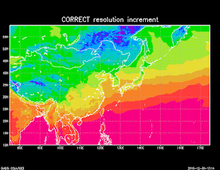
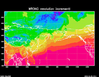
from the NETCDF file, it is inferred from the control file. So it is important that the resolution and the starting points are right, otherwise you will get an incorrect result, even if your longitude data is correct in the NETCDF file. For example, comparing the correct (0.25) resolution to an incorrect resolution (0.45) gives the two different maps shown on the right. So get the resolution right!
 One final note: This kind of control file only seems to work with nice rectangular datasets. That is lat/lon coordinates that vary independently from one another. If your lat/lon grid does not vary independently (i.e., longitude is a function of y and visa-versa), then using this method will warp tour map projection. In these situations it is recommended that you write your data out to a binary file with the PDEF option. I have yet to get the PDEF option to work with a NETCDF file.
So that is it for the tutorial, hopefully you have a better understanding regarding the difference between self describing and non self describing NETCDF files, and how to write and open them in GrADS. No GrADS scripts to download here, but a full python script (version 2.7) is included that will reproduce the files and plots generated in this tutorial. You will need the netCDF4 module installed for this script to work however. Numpy and sys are standard I believe. Also you may need to update the date.
Download Python Script here


Thank you for sharing!
ReplyDeletebut I use NCL for computing.. do you know how to use NCL create a ncfile for grads?