Script: Colormaps.gs; very easily create elegant color scales for your plots using GrADS

 NEW VERSION AVAILABLE HERE:
Version 2

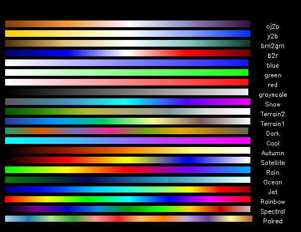
If you are a frequent visitor to this site you probably know that I focus a lot of my effort into color scales.  I often reference the color.gs script as a must have script in ones script library.  I have additionally added the script colorset.gs to the script library for use with common remote sensing color scales.  This script here is similar to colorset.gs, but different in the sense that it gives the user control as to what number scale the color map will be set to.  colormap.gs currently includes 21 color scales (with the option of reversing them).  These scales are shown below.

Colorscales included in colormaps.gs

Optional Arguments for colormaps.gs

• -demo             - Pulls up Demo page
•  -flipped          - Reverses direction of color scale
•  -name/map     - chooses colormap
•  -levels/l          - sets scale: max min int
• -help                - Pulls up help page (includes full list of color maps)

Example: Open WRF data and plot the 2 meter dew point using the  reversed "ocean" color map

  'sdfopen http://nomads.ncep.noaa.gov:9090/dods/hiresw/hiresw20140503/hiresw_eastarw_00z'
  'set gxout shaded'
  'clear'
  'set mpdset hires'
  ' colormaps -flipped -l 265 310 1 -map ocean'
  'd dpt2m'
  'cbar'

This series of commands will produce the following image.

2m Dew Point using "Ocean" colormap

This is the first version, so check for bugs and please report any you find!

Enjoy!

Download Colormaps.gs 

Download Example Script

Read More

Tutorial: GrADS Widgets, and GUI capabilities; Make a functional calculator using GrADS

This tutorial will show you how to use a few of the widgets that come with GrADS to create basic Graphical User Interfaces (GUIs).  We will use these tools, to create a functional calculator.  This exercise should familiarize you with how to make basic GUIs using the GrADS scripting language.

I have been on the fence about writing a full tutorial about GrADS widgets, as there is already a lot of good material out there describing how to use them.  Though ultimately I decided that it would be beneficial to have a more in depth tutorial that really details some of the logic involved.  So, if you are just looking for fast reference, this tutorial may be a bit much.  If you are looking for a quick reference, I encourage you to check out this site.

Before you start the tutorial, you may be thinking to yourself; "Why go through all the effort to write GUIs?"  GUIs are nice because they are what most people are familiar with, and often times I find it easier to use a GUI interface that has many preset options built in, rather than slightly editing code, or manually inputting different values into the console.  So in that respect, it is worth the upfront time and effort to write the GUI, so you can accomplish a wide variety of operations with the click of a button.

Lets get started, as always (and so you know what the end goal is), below is an image of the finished product.

Calculator GUI

In writing this tutorial, I have wracked my brain a little trying to figure out a nice way to summarize GUI structure using the GrADS widgets.  The best thing I could come up with is that when you write a GUI, you need to create the infrastructure first; the buttons, the drop menus, etc., then you need to write the functions of each individual component of that infrastructure.

The first thing we need to do is set up the infrastructure of the GUI, this will serve as sort of the skeleton that the calculator functions will work with.

To set up the GUI infrastructure, we are going to break the buttons into 4 groups.

1. Number Keys
2. Basic Operators (+ - * /)
3. Special Operators (sin/cos/etc.)
4. Other (Quit, Ce, Enter)

In addition to the GUI components, we need to include some dynamic updating of the "Display Screen."  This will be straightforward though, as we will just use the 'draw recf' and 'draw rec' commands to update the display.  Before we get to the display, we will start by going through writing each group of widgets separately.

Group 1: The Number Keys:

Since this is the first examination of the GrADS 'Button' widget, I will briefly explain the syntax used.  So the two relevant commands for the Button widget are: 'set button', 'draw button' and 'redraw button.'  The first two commands are followed by numerous arguments, the last one only requires one argument, and determines if the button is in the "on" or "off" position.

The "set button" command sets up the style of your button, the color, the text color, and the borders.

'set button' takes up to 9 arguments taking the form of:

'set button 1 15 1 1 2 15 1 1 3'

Where the first 4 arguments represent the OFF position; text color, face color, bright color for border shading, and the dark color for the border shading.  The second 4 arguments represent the same thing, but for the ON position.  The Final argument, sets the thickness of  your shaded border, with large numbers creating a noticeable 3D bevel effect, and small values basically draw a line around your button.  The above command is the style used for the calculator,  and it sets the number key buttons to be gray colored with white text when off, and gray colored with red text when on.  A few other examples are shown below.

• button1:   'set button 1 4 6 7 1 2 7 6 30'
• button2:  'set button 5 8 15 1 5 8 15 1 30'
• button3:  'set button 2 3 15 1 2 3 15 1 1'

Button Examples

Now that we have covered the 'set button' command, we need to look at the 'draw button' command.

The "draw button" command requires 6 arguments or it will send back an error.  The arguments are as follows:

1. Identifying Number
2. center in x (page coordinates)
3. center in y (page coordinates)
4. width
5. height
6. string

The most important argument is the Identifying number.  This number is how you tell this button apart from all the other buttons in the GUI.  It is important that you ensure that your buttons number is unique so that you don't have weird things happen when you click on it.  Beyond that, the remaining arguments are just for formatting purposes, setting the button boundaries as well as the string (what the user sees).

Example: 'draw button 1 5.5 5.5 1 1 Button1'
This would draw a square button, labeled Button1 in roughly the center of the GrADS display.

Now that we are familiar with the 'set button' and 'draw button' commands, we can see how to write out the number keys of our calculator.

I like to do everything inside of a loop.  Generally, if I need to execute a command more than once, I try to use a loop to reduce the amount of text I actually have to write, so that's what we are going to do here.  We are going to loop through each number 1-9, draw each row of buttons, and then draw the remaining two buttons (0 and .) on the last row.  Since this is an advanced tutorial, I will just copy down the code for the loop, and let you make sense of it.

  *Environmental Variables to set scale*
  cols=3
  nums=11
  bnum=1
  w=0.75
  xstart=3.5
  ystart=5.5
 ****

   'set button 1 15 1 1 2 15 1 1 3'
   y=ystart
  while(bnum<=nums)
    col=1
    x=xstart
    while(col<=cols)

      if(bnum<=9)
        'draw button 'bnum' 'x' 'y' 'w' 'w' 'bnum
      else
        if(bnum=10);'draw button 'bnum' 'x' 'y' 'w' 'w' 0';endif
        if(bnum=11);'draw button 'bnum' 'x' 'y' 'w' 'w' .';endif
      endif

      x=x+w*1.5
      col=col+1
      bnum=bnum+1
    endwhile
    y=y-w*1.5
  endwhile

This code, will draw all 11 buttons (0-9, and the decimal point).  The environmental variables are there so you can play with the size and shape.  Just make sure you note that each button is given its own unique identifying number, that number will come in handy later when we set up the actual functions associated with each button.  The fact that each identifying number is equal to the string also comes in handy later.

Group 2: The Basic Operators:

This code is similar the code used to write the number keys, but with minor differences.  Once again, we use a loop to write out the operators.

  cols=2
  strings='+ - * /'
  bnum=12
  nums=16
  xstart1=x
  y=ystart

  'set button 0 4 15 1 2 4 15 1'

  while(bnum<nums)
    col=1
    x=xstart1
    while(col<=cols)
      str=subwrd(strings,bnum-11)
      'draw button 'bnum' 'x' 'y' 'w' 'w' 'str
      x=x+w*1.5
      col=col+1
      bnum=bnum+1
    endwhile
    y=y-w*1.5
  endwhile  

A few important things to notice in the above code:

• We use the 'set button' command to reset the button to have a blue face
• We change the number of columns to 2
• We use a master string that has all 4 sub-strings representing each operator
• See: Tutorial on Arrays if you are unfamiliar with this
• We start the identification number (bnum) at 12 so that it doesn't interfere with the buttons already created

Group 3: Special Operators

In order to illustrate the use of the 'drop menu' I chose to include a few "special" math functions in the calculator that you would access using a nested drop menu.  So the drop menu syntax in GrADS is a little different than the 'draw button' syntax.

Similar to the button widget, the drop menu also has a formatting precursor 'set dropmenu'  This command takes up to 15 arguments, corresponding to different formatting options like text color, borders, widget color.,etc.  These 15 arguments are well described here and in the interest of time, will not be thoroughly discussed in this tutorial.  Though similar to 'set button' these values correspond to the same attributes, but under different circumstances, e.g., whether or not a given option is selected.  I'll be honest, I usually just ignore the 'set dropmenu' command and use the default options, but you could make a really slick interface with fully customized colors and borders using this command if you so chose.

The 'draw dropmenu' command is fairly straightforward.  Similar to 'draw button' it requires 6 arguments, and the first 5 are identical to the first 5 arguments for 'draw button'.  Again, be sure that your drop menus identification number is unique. The last argument is your drop menu.  It is a collection of strings that represent different options with each option separated by a "|"

Example: 'draw dropmenu 1 5.5 5.5 1.1 0.7 Menu | option1 | option2 | option3'

The string before the first "|" is what the user sees on the display when the dropmenu is not selected.

Drop menus can be nested or "cascaded" with a small addition to the string at the end of the menu.  Using the above example we can get a cascading menu from option 3 by altering it as such:

'draw dropmenu 1 5.5 5.5 1.1 0.7 Menu | option1 | option2 | option3 >10> '

This now tells your widget that you want option3 to point to a cascading drop menu with the identification number 10.  Now, we just need to set up that cascading menu.  For this, we use the 'draw dropmenu' command again, except we replace all of the spatial variables with the word "cascade."  This specifies that you want this menu to be attached to another menu.  Then, the syntax is the same, you need the identification number (in our example 10) followed by your options.

'draw dropmenu 10 cascade cascade1 | cascade2 | cascade3 '

So that it is for the basics behind the drop menu and the cascading (nested) drop menus.
Now that we know how to use the 'draw dropmenu' command, I will show you how it's used in our calculator!  This is actually easy, since we only have one drop menu in the calculator.

  x=xstart1+w*0.75
  h=w
  w=2*(w)+w*0.5

  'draw dropmenu 16 'x' 'y' 'w' 'h' Special | e^x | x^2 | ln(x) | Trig >03> '
  'draw dropmenu 3 cascade sin(x) | cos(x) | tan(x) '
  
First we simply reset the location and size of the drop menu relative to the rest of the calculator, then we just draw the drop menu.  Notice that the parent drop menu has a unique identifying number, but the nested menu does not.  This is because the identification for the cascading menu is in a different spot than the identification for the parent, so this does not need to be unique (More on this soon).


Group 4: Other

The last group, the other important buttons; Enter, Clear (CE) and Exit and the display.  The exit button is important as it will break the loop within the GUI, more on this when we build in the GUI functionality.  But since there is nothing particularly new here, I'll just give you the code, and you should be able to see what it is doing.

Starting with the Display:

recxlo=xstart-w*0.5
recylo=ystart+0.75
recxhi=xstart+w*4.5
recyhi=ystart+1.75

'set line 1 1 1'
'draw recf 'recxlo' 'recylo' 'recxhi' 'recyhi

'set line 15 2 6'
'draw rec 'recxlo' 'recylo' 'recxhi' 'recyhi

The display just draws a couple of rectangles above the button interface.

Then the Buttons:

ymid=(recyhi+recylo)/2
xmid=recxhi+0.75
y=y-h*1.5

'draw button 100 'xmid' 'ymid' 'w*1.25' 'w*1.25' CE'
'draw button 101 'recxlo+w*0.625' 'y-1.25' 'w*1.25' 'h' Quit'
'draw button 102 'recxlo+w*2.20' 'y-1.25' 'w*1.25' 'h' Enter'

And that should draw out the full calculator!  If you haven't done so already, now may be a good time to take a quick break.  Below we move away from building the infrastructure and get into designing the functionality to our calculator.

The entire functionality of the GUI interface is based on the 'q pos' command.  This command prompts the user to click somewhere on the display screen and returns information including the page coordinates, mouse button, and widget properties.  More details on the 'q pos' command can be found here.

The basic design we will use is a loop that keeps prompting the user to click on the screen until the 'quit' button is pressed.  Within the loop is where the magic happens.  So we first set up the loop, with the condition for exiting.  Before we start the loop, we need to set up a few initial conditions.  Since the calculator performs math operations on two numbers, we will need two numbers for variables, and a variable for the returned number. Lastly, we need a variable that represents the operator.  So we do that before the loop.

  calculated=0
  num1=''
  num2=''
  op=''

  while (1)
    'q pos'
    num = subwrd(result,7)
    if (num=101); break; endif;

This sets up the initial conditions and starts the loop, and gathers the information about which button you are pressing using the 'subwrd()' function. Remember, the 'Quit' button identifier is 101, so we set the condition that if the returned button is 101, we break the loop.

Now, lets write down the code that sets up the numbers.  I'm going to just show the code, and explain it after.

  if(num !=-1 & num!=16 & num!='')

    'redraw button 100 0'
    'redraw button 101 0'
    'redraw button 102 0'

    if(num<12)

      if(num<10);out=num;endif
      if(num=10);out=0;endif
      if(num=11);out='.';endif

      if(op='')

        num1=num1''out
        'set line 1 1 1'
        'draw recf 'recxlo' 'recylo' 'recxhi' 'recyhi
        'set line 15 2 6'
        'draw rec 'recxlo' 'recylo' 'recxhi' 'recyhi
        'draw string 'recxhi-0.25' 'ymid' 'num1
      endif

      if(op!='')

        num2=num2''out
        'set line 1 1 1'
        'draw recf 'recxlo' 'recylo' 'recxhi' 'recyhi
        'set line 15 2 6'
        'draw rec 'recxlo' 'recylo' 'recxhi' 'recyhi
        'draw string 'recxhi-0.25' 'ymid' 'num2

      endif
    endif

We start first with the condition that num is equal to something, and something other than the dropmenu.  This sets it so that you can click all over the screen as many times as you want and nothing will happen.  We then reset all of our miscellaneous buttons to the off position (this is purely for formatting, the actual button status is not used in any of the functions).

To get the functionality of the buttons, we start by checking the condition that the num<12.  This checks whether or not you are adding a number, or doing something else.  Within that condition, there is the check for whether or not there is an operator set.  Since we want to make this like a real calculator, if an operator is set, we put our numbers into num2, and if it isn't we put it into num1.  We set numbers by concatenating strings, so you just keep pressing numbers to build up your number.  We also need to distinguish if we add a number, or a 0 or a decimal point.  Once our number is changed, we wipe the display and redraw it with the chosen number.  This happens so fast, that it appears as if you are just entering numbers into the calculator.

Next, we need to set up the operators.  To keep things simple, and since there is already a conditional statement isolating the drop menu, we'll first stick with the first basic operators.

    if(num=12);op='+';endif
    if(num=13);op='-';endif
    if(num=14);op='*';endif
    if(num=15);op='/';endif


    if(num>=12 & num<=15)
      bcount=1
      buttons=11
      while(bcount<=buttons)
        'redraw button 'bcount' 0'
        bcount=bcount+1
      endwhile
    endif

This code just uses a bank of conditional statements to set the operator up.  Once the operator is set up, and as long as you have selected a basic math operator the program loops through and sets all numbered buttons to the off position.  Next up, the special operators.  Note: This code is a little out of position, since the code that makes the calculations is within the conditional that excludes num=16.  But it seemed to make more sense in this order for the tutorial.

  if(num=16)
    special=subwrd(result,8)
    if(special=4)
      special=subwrd(result,10)+10
    endif

    if(special=1);op='exp';endif
    if(special=2);op='pow';endif
    if(special=3);op='ln';endif

    if(special=11);op='sin';endif
    if(special=12);op='cos';endif
    if(special=13);op='tan';endif

    'set line 1 1 1'
    'draw recf 'recxlo' 'recylo' 'recxhi' 'recyhi
    'set line 15 2 6'
    'draw rec 'recxlo' 'recylo' 'recxhi' 'recyhi
    'draw string 'recxhi-0.25' 'ymid' 'op'('num1')'

  endif

Since the drop menu identifier is in a different location when 'q pos' is called, we need get the drop menu identifier first.  We then need to check if the drop menu is equal to the cascade, in which case, we need to get the cascade option.  I add 10 to easily differentiate from the other values.  Then, we just set the op to the special values, and display the operator on the screen.

Finally, we are almost done.  Now we have all of our information, and we are ready to calculate our numbers!  Going back into the conditional statement that excludes num=16.  We start with the conditional value of 102 (the 'Enter') button.

    if(num=102)
      if(op!='')
        if(num1='');num1=0;endif
        if(op='+');calculated=num1+num2;endif
        if(op='-');calculated=num1-num2;endif
        if(op='*');calculated=num1*num2;endif
        if(op='/');calculated=num1/num2;endif


***     ***SPECIAL OPERATIONS****

        if(op='exp');calculated=math_exp(num1);endif
        if(op='pow');calculated=math_pow(num1,2);endif
        if(op='ln');calculated=math_log(num1);endif

        if(op='sin');calculated=math_sin(num1);endif
        if(op='cos');calculated=math_cos(num1);endif
        if(op='tan');calculated=math_tan(num1);endif

        num1=calculated
        num2=''

       'set string 0 r 6'
       'set strsiz 0.2
       'set line 1 1 1'
       'draw recf 'recxlo' 'recylo' 'recxhi' 'recyhi
       'set line 15 2 6'
       'draw rec 'recxlo' 'recylo' 'recxhi' 'recyhi
       'draw string 'recxhi-0.25' 'ymid' 'calculated

        op=''
        bcount=1
        buttons=12
        while(bcount<=buttons)
          'redraw button 'bcount' 0'
          bcount=bcount+1
        endwhile

        bcount=12
        buttons=16
        while(bcount<=buttons)
          'redraw button 'bcount' 0'
          bcount=bcount+1
        endwhile

      endif
    endif

This code looks long, but it's more of the same.  The only thing new is the block of conditional statements that performs the calculations based on what operation you have in place.  Then you set num1 to the calculated value, so you can continue to make calculations using the newly calculated number.

Now, we have one last loose end to tie up before we are finished with the calculator.  The 'Ce' button.
This button is designed to reset all the initial conditions, and redraw the display.

    if(num=100)
     num1=''
     num2=''
     op=''
     calculated=0

     'set line 1 1 1'
     'draw recf 'recxlo' 'recylo' 'recxhi' 'recyhi
     'set line 15 2 6'
     'draw rec 'recxlo' 'recylo' 'recxhi' 'recyhi
     'draw string 'recxhi-0.25' 'ymid' 0'
    endif
 endwhile

That about does it!  You now have a working calculator!  More importantly, you should have a pretty good foundation in creating GUIs in GrADS using the 'button' and 'drop menu' widgets.  If you followed the code segments throughout the script, it may be difficult to get a working script together due to some of it being out of order.  It is therefore recommended that you download the script provided, and edit that as you please.

I recommend that you play around with this script, change button styles, add or subtract special functions, etc.  I hope you enjoyed this tutorial, and hopefully you learned something about using GrADS widgets.  As always, feedback is much appreciated.


Download Example Script Here 

Read More

Tutorial: Overlay model resolution onto weather map

There may come a time in your professional or student career when you will have to show a model grid overlaid on a map, to illustrate some sense of your model grid size.  This approximation can be done fairly easily in GrADS using a little bit of spherical geometry, a couple of while loops, and the 'q w2xy' command.

This tutorial will show you how to do this using the topography file from the Grads Data Server.
When you are finished with this tutorial, you will be able to reproduce the plot below.

40km grid overlaid on southwest US.

The first step in this process is to get that data.  One we have the data we set up the domain and do a little formatting.

   file='http://www.monsoondata.org:9090/dods/topo/rose/etopo05'
   'sdfopen 'file
   'set mpdset hires'
   'set display color white'
   'clear'

Now that we have our file open (and if you want, you can do a 'q file' to see the details), since we are plotting over an area bigger than the area we are drawing our model grid on, we need two sets of lat/lon boundaries.  The next bit of code provides the coordinates for the example plot, but you could of course choose your own boundaries.  I like to set these before hand, for easy changes later on.  In addition to your lat/lon boundaries, you need to choose a model resolution.  Once again, I just set this as a variable rather than "hard coding" it in, for quick access to changes.

  lat_bound='32 41.5'
  lon_bound='-115.5 -105'

  lat='32.5 40.25'
  lon='-115.0 -105.5'

   res=40000

Now that we have our initial conditions set, we can move on to plot the topography.  In this example, I use the script checkered.gs, available in the script library, to plot the nice boarder.  So I want to turn the x/y labeling off.  If you have read any of my other tutorials you'll already know this, but I use color.gs to set the color scale.  So if you have these two scripts in your script folder, you can follow along, with the code below.  If not, you can still follow the tutorial, just without the boarder and color scheme.

  'set xlab off';'set ylab off'
  'set gxout shaded'
  'set grads off'
  'set lat 'lat_bound
  'set lon 'lon_bound

  'color 50 5200 100 -kind green->tan->dimgray'
  'd rose'

The above code plots the topography from the topography file.  Remember, when setting the lat/lon boundaries to use your outer boundaries.  So that your inner box will fit inside.

This next part introduces the use of the 'q w2xy' command: World (w) to (2) x/y (xy).  Basically, you are translating lat/lon coordinates to page coordinates.  Before we plot the grid, we are going to first approximate the domain, and I use the term "approximate" because it won't be exact due to the fact that the physical distance between longitudinal coordinates is dependent on latitude, so the simple rectangle isn't an exact representation of the world coordinate system.  Anyway, we simply take the inner lat/lon boundaries and the the lower-left and upper-right corners using 'q w2xy' and then we draw a rectangle using the 'draw rec' command. 'Set line' is used to do a bit of formatting (e.g., the blue color in the example image).  A more detailed explanation of how to do this part is provided in this tutorial

  'q w2xy 'subwrd(lon,1)' 'subwrd(lat,1)
  xpos1=subwrd(result,3);ypos1=subwrd(result,6)

  'q w2xy 'subwrd(lon,2)' 'subwrd(lat,2)
  xpos2=subwrd(result,3);ypos2=subwrd(result,6)

  'set line 4 1 8'
  'draw rec 'xpos1' 'ypos1' 'xpos2' 'ypos2

Now we are ready to draw our model grid.  There are more than a few ways to go about doing this, and  the main thing is you want to get your starting and ending lat/lon points set.  Then we want to set up the constants that we will use in our spherical geometry calculations.  For all intents and purposes, we assume the distance per degree of latitude (mperlat) is constant. While it does have some variation due to the not quite spherical shape of the Earth, it's not a bad assumption that it's constant.

  latstart=subwrd(lat,1);latend=subwrd(lat,2)
  lonstart=subwrd(lon,1);lonend=subwrd(lon,2)

 mperlat=111200
 r_earth=6378000
 pi=3.141592

So, now we have our boundaries set, and our constants we can start to draw our grid.  So the basic idea is that we loop through all longitude and latitude points drawing boxes with sides roughly equal to our resolution.  There are several levels of complexity that can be used to approximate the distance per degree of longitude.  This tutorial will focus on the most simplistic way, however it will touch upon some of the more complex ways to go about it.

The simplest way to approximate your zonal grid resolution, is to just set one value for "delta_lon" for the whole grid, and apply that throughout.  The best way to do this, would be to take a mean latitude for your domain, and calculate delta_lon from that.  So setting delta_lon and delta_lat is reduced to:


   avg_lat=(latstart+latend)/2
   delta_lon=(res/r_earth)*(180/pi)/math_cos(avg_lat*pi/180)
   delta_lat=res/mperlat

This approximation is pretty good, so long as you are at low to mid-latitudes, and your domain is small. Usually when illustrating your model grid, you want to keep the domain small so that you can see the boxes better (unless your resolution is 200km or something like that, in which case you have bigger problems).  So this approximation isn't bad.  Now that we have delta_lat and delta_lon, we just loop through and draw boxes.  I like to start with my grid-box centered on my lower-left corner, so before entering the loop, I do a quick adjustment to my latstart, and lonstart.  Remember, to reset your starting longitude value within your latitude loop.

   'set line 2 1 1'        ;*Formatting
   latstart=latstart-delta_lat/2

   lat=latstart   
   while(lat < latend)

     lat1=lat
     lat2=lat1+delta_lat
     lon=lonstart-delta_lon/2

     while(lon < lonend)
       lon1=lon
       lon2=lon1+delta_lon


       'q w2xy 'lon1' 'lat1
        xpos1=subwrd(result,3);ypos1=subwrd(result,6)

       'q w2xy 'lon2' 'lat2
        xpos2=subwrd(result,3);ypos2=subwrd(result,6)

       'draw rec 'xpos1' 'ypos1' 'xpos2' 'ypos2
       lon=lon+delta_lon
    endwhile
    lat=lat+delta_lat
  endwhile


That's all there is too it!  You simply use a nested loop set up, to loop through all longitude and latitude values, drawing boxes first in the x-direction, and then in the y-direction.  Now, if you want the nice border around the plot, simply call the 'checkered.gs' script (again more information on this, can be found in the GrADS-aholic! script library).

  'checkered  -s 1.0 -w 0.1 -ss 0.09'

And, you will have your plot.

Now, as mentioned you can get more complex with setting the delta_lon values.  For example, you could re-calculate delta_lon as you loop through latitudes, taking the average latitude value to be the average of each grid-box.  Essentially, you recalculate delta_lon inside of the latitude loop, rather than use the same one for the whole domain.  If you really want to get fancy, you could calculate a delta_lon at the bottom of and the top of your box.  In this case, you are no longer able to use the 'draw rec' command, because you are dealing with 4 unique points, rather than a simple rectangle.  So you would need to use the 'draw line' command to draw your borders.  These methods are better used if you are near the poles, or using large domains, and they are simply trying to refine your approximation of distance between longitude points, and essentially account for the fact that your distance between degrees of longitude decreases as you move to high latitudes.

I hope you enjoyed this tutorial and found it worth while.  As always, a link to a script with this tutorial in it is provided.

Download Example Script

Read More

Tutorial: An introduction to using surface station data in GrADS

In addition to plotting gridded data, GrADS can also be used to plot station data; that is data formatted with information specified at specific latitude/longitude coordinate rather than data gridded in a mesh that spans a region. This tutorial will show you how to use some of the functions in GrADS to work with surface data from both the mesonet and METAR inventories to generate surface maps with and without contoured data. At the end of the tutorial, you will know how to make the images shown below using station data. 

Surface map with METAR data.

Surface data and Contoured Sea level Pressure From METAR data

Surface data and Contoured Sea level Pressure From METAR data

First things first: Getting the station data.  Getting the station data and, more importantly, getting it into the right format is the trickiest part of using station data with GrADS.  To get the data into the right format, you must have knowledge of coding in another language (Fortran, C, Python, etc,.).  The scope of this tutorial is to focus on using the station data in GrADS, and not showing you how to get the data into the right format.  So if you are looking to learn how to format station data such that it can be read into GrADS, this tutorial is not for you. 

Some good information regarding how to format station data can be found here and here.  The basic idea is that you need to take the station data, write out a binary file with a header including information such as station id, latitude and longitude, and then the actual data for each station.  Afterwords you need to write out a control file to tell GrADS how to interpret your binary file.

Since I am not going to show you how to grid station data, I have prepared a few files for you to use with this tutorial.  They can be found here:

Mesonet Data (for temperature map)

• mesotest.ctl
• mesotest.dat 

 METAR Data (For station and SLP maps)

• metartest.ctl
• metartest.dat
  

Once you have downloaded these files and placed them in your GrADS directory (note: Mine is c:/OpenGrADS/, you may need to change the 'dset' variable in the .ctl files to match your GrADS directory).  Now before you can open the file, you need to use the 'stnmap' utility to help map out the data.  This is easy enough to do.  Before you open GrADS, open up a console (windows command prompt) and type the following command to make your station map.

    'stnmap -i mesotest.ctl'     ---> For the mesonet data.

    'stnmap -i metartest.ctl'    ---> For the METAR data.

This makes your station data accessible in GrADS.  For more information on the station map utility you can read more here.

Now you are ready to open up GrADS!  We'll focus on the station data only first.  To do this start by opening up metertest.ctl, and do a 'q file' to see whats in the data.

    ''open metartest.ctl'

    'q file'

This will tell you what variables are in the file.  In the data file provided, cld and wxsym are dummy variables and contain no relevant information;  they are just place holders.  What we are going to do is plot out station plots with temperature and dew point.  This is very simple, all that is needed is to first 'set gxout model' and then display the data.  To commands below will reproduce the first image seen (without the title).

    'set display color white'
    'set mpdset hires'
    'clear'
    'set lat 30.52 40.24'
    'set lon -100.39 -90.11'
    'set gxout model'
    'd u;v;ts;td'

The 'd u;v;ts;td' tells GrADS to plot a station model with wind components u and v, along with the surface temperature and dew point.  Note: without u;v components nothing will plot when the graphics is set to 'model'.  To add more, you simply increase the number of variables in the chain (in proper order).  For example to add SLP the command would be: 'd u;v;ts;td;slp'.  Missing variables are represented by a 0.0.  The expected order of variables is well described here.

Now lets say we want to do a similar station plot, only now with the contoured sea-level pressure.  To do this, you need to fit your station data to a preexisting grid.  In this tutorial, we will use the RAP model as our base grid.  It doesn't matter which data set you use, but it is recommended you pick something that is of similar grid spacing to your station plot (e.g., it wouldn't be good to use grid METAR data to 2km grid spacing).  Since we are using METAR data, the commands will be almost the same as the ones above with the only difference being a domain change.

    ''open metartest.ctl'

    'set display color white'
    'set mpdset hires'
    'clear'
    'set lat 36 49'
    'set lon -84 -65'
    'set gxout model'
    'd u;v;ts;td'

Once this is done, we need to open up the RAP model data using the 'sdfopen' command.

   'sdfopen http://nomads.ncep.noaa.gov:9090/dods/rap/rap20140216/rap32_12z'

This file is now open as file 2.  From here it is simple, we just use the oacres function to fit the data to the grid.  Now here, it does not matter which variable from the RAP you use, since it is just a dummy variable to get the grid to which the station data will be interpolated too using the Cressman objective analysis on. 

First some formatting...

    'set cthick 6'

    'set clevs 990 994 998 1002 1006 1010 1014 1018 1022 1026 1030'

    

Then we can use the oacres function to interpolate the station data.

    'd oacres(rh2m.2,slp.1,45,30,20,10,5)*33.86'

And voila, you have your station SLP contoured on your map.  To break down what exactly is going on in the above command:

The first argument (rh2m.2) is the variable from the RAP model, essentially the grid you are projecting your data onto.  The suffix .2 is simply there to specify that you want the variable from file number 2 (if you are unfamiliar with how to handle multiple files in GrADS, check out this tutorial).  The second argument (slp.1) is the station variable you want interpolated to the grid, in this case Sea Level Pressure.  The arguments after that specify different radii of influence that you are using to interpolate the station data with.  This will take a little experimentation on your part to get right, but the selection used above seemed to work fairly well with this data set.  I am personally not 100% familiar with the exact math behind the Cressman OA, so if you want to know more on that, you are on your own.  The factor of 33.86 is to convert the station SLP reported in inHg to mb.

The final lesson in this tutorial is very similar to the 2nd lesson except now, we are using mesonet data, which has a higher density than METAR data.  So again we will start by opening the file (in this case the mesotest.ctl).

    'open mesotest.ctl'

    'set mpdset hires'
    'clear'
    'set lat 36 49'
    'set lon -84 -65'

Instead of displaying the data as a station model, we are doing a shaded contour underneath the station data.  So we need to do the Cressman OA first, which means we need to open the RAP file and set up our formatting.  In this example, I used color.gs and xcbar.gs to set the color scale and color bar, but you can do that however you would like.

  'sdfopen http://nomads.ncep.noaa.gov:9090/dods/rap/rap20140216/rap32_12z'
  'color -20 100 2 -kind fuchsia->darkblue->lime->yellow->red'
  'set gxout shaded'
  'd oacres(rh2m.2,ts.1,45,30,20,10,5)'
  'xcbar 10.10 10.20 0.5 8.0 -fs 5 -line on'

This will draw your shaded station temperature data fit to the RAP grid.  Once again, you may have to play with the radii numbers to get it exactly to your liking.  Same goes for your color location and your color scale.  Once this is done, simply use the 'set gxout value' command and display your temperature data.

  'set gxout value'
  'd ts'

And that about does it for your temperature plot, and for that matter, this tutorial!  I hope you enjoyed it and found it interesting.  The script below has the examples described here and is set for you to use and experiment with.  

As a final note:  The station ids were not plotted with the data in the examples in this tutorial.  However, this can be toggled in GrADS by using the 'set stnid' command.  For example, to turn on the plotting of the station ids: 'set stnid on' .   

Thanks again for reading!

Download Example Script

Read More