Script: diamondbar.gs; Draw a colorbar using diamond shapes on your plots.

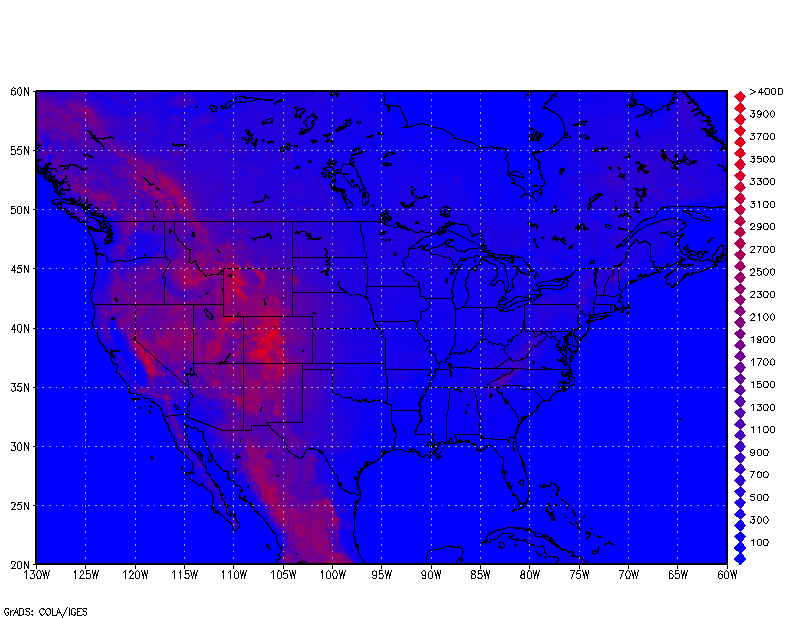
I have not added anything to this blog as of late, I have been busy with a number of different projects including my participation in the OWLeS field project.  Recently I have seen a few presentations that showed figures that had color bars made up of diamonds rather than rectangles (see below).  I figured it might be fun to put together a quick script that allows you to do this in GrADS.

Colorbar with diamonds using diamondbar.gs

Example usage:
            'diamondbar -r -marg 0.1 -font 0.09 -fs 2'

This is the call used to plot the colorbar on the above example. 

Options:        -help           - Pulls up this Help Page
                       -loc             - Chooses location for the colorbar (r=right-vertical,                                                                            l=left-vertical, b=bottom-horizontal,t=top-horizontal)                                                                             can also be called by (-l,-r,-b,-t)'
                        -size/s        - sets size of each diamond, defaults to "auto"
                        -marg            - sets margin to axis
                        -fs/int         - sets the interval for each number plotted along the colorbar
                        -font/fontsize  - sets the font size of the numbers
                        -scol           - sets the color of the numbers
                        -line           - draws outline around each diamond if included  


Anyway, I had some free time recently, and I got inspired to write a new script, so I quickly put together this script.  I haven't used it too much, but I certainly see how and where it could be useful, perhaps to add a little flare to your figures.  Enjoy!  And as always, report any bugs!

Note:  The example script will generate the plot above and requires the script color.gs

Download diamondbar.gs

Download Example Script

Read More

Script: Boxplot.gs; Make Box Plots from user-input data.

I wrote this script after I finished the script statpack.gs since most of the heavy lifting was already finished.  Boxplot takes data from a user input array in the form of a string with array elements separated by spaces (same as scatter.gs) and plots out a box plot using that data.  To use this script, no outside file is required.  It is written such that an unspecified number of box plots can be plotted on the same plot.  In most cases, this type of analysis is best left to other plotting software, but this script may be of some use in certain cases.

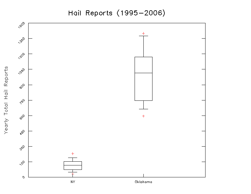
Example usage: Hail Reports between 1995 and 2006.

    array1='64 88 127 49 175 115 128 31 190 82 229'
    array2='712 595 663 777 795 1400 1375 1029 1256 1083 1015 '
    'boxplot -d 'array1' -d 'array2' -range 0 1500 -enclose -cap -title -ytitle -xlab custom'

Example of Boxplot.gs output: Hail Reports.

This example is for the number of small hail reports in New York and Oklahoma.
As you can gather from the above example, this script takes a whole bunch of arguments, all are listed in a help section and can be set at the top of boxplot.gs.  I had other examples to present involving climatology data, but the government shutdown has made accessing this data a bit frustrating, so that has been tabled for now.  For more information on how to populate an array from data contained in a GrADS .ctl file, check out the example on scatter.gs.

Notes:

• This script can process as many arrays as you specify, as long as each array is preceded by a "-d"
• Unlike scatter.gs I did not spend a lot of time on "anti-clipping", so if you specify your data-axis (rather than leaving it on auto) you may find your data exceeding your boundaries.
• Similarly, the larger you set your boxsize, the more likely your data might exceed your plot boundaries (a boxsize <0.1 is recommended)
• The data represents the inner-quartile-range, the median, and the lines extend to the 10th and the 90th  percentile [calculated using the formula used by MS Excel - q=p*(n-1)+1].
• If you turn on title plotting (-title) in your arguments, you will be prompted to enter your title, so be sure to keep an eye on your console for instructions.

Hopefully you find this script useful, this is v1.0 so be on the lookout for bugs, I have tested most of the options and I can't see any bugs as of now, but if you find some, please report them here!

Download Boxplot.gs

Download Example Script

Read More

Script: Statpack; Perform basic statistical analysis on user-input arrays.

This is another one of those scrips that extends the flexibility of GrADS beyond it's intended purpose.  As usual, these analyses might better be performed using higher level data analysis software (e.g., python or matlab).  However, this script might be useful for generating quick statistics on data sets that are in GrADS format without the intermediary step of saving data to a file to read into another program.


This script is not a script that you call, but instead a library of functions that you include in your script.  Note: you must include all functions as some of these functions rely on each other to operate.

In order to use this script, your data arrays must in in the format of strings with your array elements separated by spaces.  e.g., array='1 2 3 4 5 6 7 8 9 10'.

Each function requires different inputs.  A list of the included functions is below, as well is in a brief help page at the top of the script.

Function list

• mean(arr): Returns mean of input array "arr"
• stdev(arr): Returns Standard Deviation of input array "arr"
• sort(arr): Returns sorted array (lowest to highest) of array "arr"
• rank(arr): Returns an array size equal to array "arr" ranging from 1 to size(arr)
• percentile(arr,p): Returns the data percentile (p) of array "arr"
• size(arr): Returns the number of elements in array "arr"
• max(arr): Returns the maximum value in array "arr"
• min(arr): Returns the minimum value in array "arr"
• correlation(arr1,arr2): Returns the correlation coefficient "r" between "arr1" and "arr2"
• regression(arr1,arr2): Returns the regression coefficient between "arr1" and "arr2

Example Use: 

•  Calculate median of array: data='9 7 8 6 5 4 3 2 1' 

           median=percentile(data,0.5)
           say median
 
           Outputs "5" to screen

• Sort array: data='9 7 8 6 5 4 3 2 1' 

          sorted=sort(data)
          say sorted
  
          Outputs "1 2 3 4 5 6 7 8 9" to screen


Download statpack.gs

Read More

Tutorial: Using the fwrite command to save a subset of data.

At some point, you may find it useful to be able to grab a subset of data from a larger data set, or from multiple data sets, and put it all in a custom GrADS data file with a matching control file.  Luckily GrADS makes this possible through the use of the 'fwrite' function.  I have decided to do a tutorial on this after some experimentation prompted by a few recent discussions.  This tutorial should help you through the basics of using the 'fwrite' function in GrADS to save a subset of data into a new data file, and then write out a .ctl file to open your new data file.

Before we get started with the step by step instruction, lets take a quick look at the 'set fwrite' command in GrADS.  This command gives you the options regarding the binary output you are putting in your file.  I have played with these different options a little bit and so far I have not seen any difference in the result, so I have only been working with the fname option.  Computer scientists may know better how to use the additional options.  A full list of options can be found here.

Now, we can get into the step by step directions.  As always we are first going to start by opening a file. 

    'sdfopen http://nomads.ncep.noaa.gov:9090/dods/gfs/gfs20130915/gfs_00z'

Now this next bit is optional, but basically I want to set my dimensional boundaries dynamically, so I want to read this information directly from the parent .ctl file.  You can of course set all of these values manually and vary them to customize your data subset as you see fit.

  'q ctlinfo'
  xdef=sublin(result,5)
  ydef=sublin(result,6)
  zdef=sublin(result,7)

  xi=subwrd(xdef,4)          ; *Initial x
  xpts=subwrd(xdef,2)       ;*Total x points
  dx=subwrd(xdef,5)          ;*delta x

  yi=subwrd(ydef,4)          ; *Initial y
  ypts=subwrd(ydef,2)       ;*Total y points
  dy=subwrd(ydef,5)          ;*delta y

  zpts=subwrd(zdef,2)       ; *total z points

  x=1
  count=8
  while(x=1)
    check=sublin(result,count)
    if(subwrd(check,1) = 'tdef')
      x=0
      tdef=sublin(result,count)
    endif
    count=count+1
  endwhile
 
  tpts=subwrd(tdef,2)          ;*Total Time
 dt=subwrd(tdef,5)             ; *Delta T

  'q dims'
  timeline=sublin(result,5) 
  ti=subwrd(timeline,6)     ;*Initial Time


The block of code above, while it looks long is just setting up the dimension limits to use when calling 'fwrite' and writing the matching .ctl file. The loop is in place to account for the fact that different data sets will have different numbers of levels and that the line corresponding to time will vary between data sets.

Now that our dimensions are set, we are ready to write our data file.  In this example, I will show you how to write two variables at varying levels for a number of time steps.  The variables chosen will be Relative Humidity, and Precipitation Rate.  These can obviously be changed.  The first thing we do is use the 'set fwrite' command to specify our output file.

  'set fwrite mydatafile.dat'

Now, we can set up our dimensions and display our data. 

  'set gxout fwrite'
  'set x 1 'xpts
  'set y 1 'ypts

This sets up our dimensions to encompass the entire horizontal domain.  Now we simply loop through all desired time steps, and all desired levels, setting our levels dynamically as we go for simplicity in writing the .ctl file.

  t=1
  while (i <= 5)
    'set t ' i
    z=1
   levs=''

   while (z <= zpts)  ;*Run through all z points
      'set z 'z
      'q dims'
      level=sublin(result,4)
      lev=subwrd(level,6)
      levs=levs''lev' '  ;*Build a list of levels from the dimensions.  This will go in the .ctl file.
     'd rhprs'             ;*write out relative humidity
     z=z+1
  endwhile
 
* Var 2 (pratesfc) is only a surface variable, so it is only run through once.
 
  z=1
  while (z <= 1)
     'set z 'z
      'd pratesfc'      ;*write out precipitation rate
      z=z+1
   endwhile
   t=t+1
  endwhile 
 
  'disable fwrite'
 
Okay, so the above block of code is pretty much all you need to write out your GrADS data file.  Because you used the 'set gxout fwrite' command, when your display your variable, it won't actually show it on screen, just write it to the file specified by 'set fwrite'.  The trick here is knowing what order to display things.  The way that I have found it to work is by setting time as the parent loop, then variables, and then levels.  For example:

T=1, Time
     Var=1, Vars
         Level=1, Levels
            'd var'
        endloop
    endloop
endloop

In the example here, I simply ran through the variables one at a time inside of the time loop, but the above sequence is good generically.  I used precipitation rate to show that you can also include variables that don't have data at all levels with variables that do.

So, now that that .dat file is made, you need to write out a corresponding .ctl file so you can work with it in GrADS.  This step is pretty simple if you know how to work with .ctl files (if you don't I recommend checking out this page).  The code below shows you how to write out a .ctl file for the example here.

  write (myctlfile.ctl,'dset   ^mydatafile ')
  write (myctlfile.ctl,'undef  1e+20 ')
  write (myctlfile.ctl,'title My Test Control File')
  write (myctlfile.ctl,'xdef 'xpts' linear     'xi'  'dx)
  write (myctlfile.ctl,'ydef 'ypts' linear   'yi'   'dy)
  write (myctlfile.ctl,'zdef 'zpts' levels  'levs   )
  write (myctlfile.ctl,'tdef 5 linear  'ti' 'dt   )
  write (myctlfile.ctl,'vars  2 ')
  write (myctlfile.ctl,'rh 'zpts' 11,100  Relative Humidity       [%] ')
  write (myctlfile.ctl,'prate 1 11,100  Precip Rate       [kg m-2 s-1] ')
  write (myctlfile.ctl,'endvars')

Basically, you need to tell it to point to your data file, define your undefined values (this can be checked with your parent .ctl file), and then list your dimensions and variables.  A lot of the variables in this example are set dynamically, so you don't have to fudge around with things too much, but usually when you write these out you need to make sure that your dimensions match up to what you actually write out, or you will see some really goofy things.  Be sure not to forget the number of levels after each variable in the vars section.

That should about do it for this tutorial, hopefully this gets you started.  I personally like to use this to grab online data and place it into a local .ctl file for more intensive processing as things move faster locally.  Thanks for reading!

Download Example Script

Read More